Probability and Bayesian networks

This lecture builds the probability base for generative models: joint, marginal and conditional distributions, the chain rule and Bayesian network factorization. It works through the weather table and the loan and disease numericals. After this page you can factor a joint distribution from a DAG and apply Bayes rule by hand.

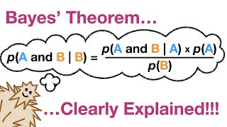Bayes Theorem Geometry3Blue1Brown · Bayes rule updating beliefs

Bayes Theorem Clearly ExplainedStatQuest · Bayes rule derivation examples

Conditional ProbabilitiesStatQuest · Joint marginal conditional probability

Joint, marginal and conditional probability Search on YouTube

A random variable names an uncertain quantity. $S$ means sunshine and $R$ means rain. Uppercase $S$ is the variable. Lowercase $s$ is one value of that variable.

The slides define three probabilities. Marginal probability is the probability of one variable. Joint probability is the probability of several variables together. Conditional probability is the probability of one variable when another value is known.

P(S, R) = P(S = s, R = r) \text{ for each cell}

$P(S, R)$ is the full joint table. $P(S = s, R = r)$ is one cell in that table. The joint table holds all the information. It is the central source of truth.

P(S = s) = \sum_{r} P(S = s, R = r) \qquad P(R = r) = \sum_{s} P(S = s, R = r)

$P(S = s)$ is the marginal of $S$ . $P(R = r)$ is the marginal of $R$ . Each marginal sums the joint cells that share its value.

P(S \vert R) = \frac{P(S, R)}{P(R)} \qquad P(R \vert S) = \frac{P(S, R)}{P(S)}

$P(S \vert R)$ is the conditional of $S$ when $R$ is known. $P(R \vert S)$ is the reverse. Each conditional selects matching rows and normalizes them to sum to 1.

Think of a full count table. Marginal adds along a row or column. Conditional zooms into one row or column and rescales it to 100 percent.

Weather table Search on YouTube

The slides use two Boolean variables $S$ and $R$ . Each pair $(S, R)$ is one possible state of the world. The joint table below matches all slide numbers. Its $R = 1$ column holds $0.08$ and $0.02$ .

$S$ \ $R$	$R = 0$	$R = 1$	Marginal $P(S)$
$S = 0$	$0.70$	$0.08$	$0.78$
$S = 1$	$0.20$	$0.02$	$0.22$
Marginal $P(R)$	$0.90$	$0.10$	$1.00$

Worked example. Marginalize the weather table.

Step 1. Marginal of $S$ . Add across each row.

\begin{aligned} P(S = 0) &= 0.70 + 0.08 = \mathbf{0.78}\\ P(S = 1) &= 0.20 + 0.02 = \mathbf{0.22} \end{aligned}

Step 2. Marginal of $R$ . Add down each column.

\begin{aligned} P(R = 0) &= 0.70 + 0.20 = \mathbf{0.90}\\ P(R = 1) &= 0.08 + 0.02 = \mathbf{0.10} \end{aligned}

Step 3. Check.

\begin{aligned} 0.78 + 0.22 &= \mathbf{1.00}\\ 0.90 + 0.10 &= \mathbf{1.00} \end{aligned}

Recompute gives the same row sums $0.78$ and $0.22$ . Recompute gives the same column sums $0.90$ and $0.10$ .

Worked example. Condition on rain: $P(S \vert R = 1)$ .

Step 1. Select the matching column.

\begin{aligned} P(S = 0, R = 1) &= 0.08\\ P(S = 1, R = 1) &= 0.02\\ P(R = 1) &= 0.08 + 0.02 = 0.10 \end{aligned}

Step 2. Normalize by $P(R = 1)$ . Divide each cell by $0.10$ .

\begin{aligned} P(S = 0 \vert R = 1) &= 0.08 / 0.10 = \mathbf{0.80}\\ P(S = 1 \vert R = 1) &= 0.02 / 0.10 = \mathbf{0.20} \end{aligned}

Step 3. Check.

0.80 + 0.20 = \mathbf{1.00}

Recompute gives $0.08 / 0.10 = 0.80$ . Recompute gives $0.02 / 0.10 = 0.20$ . The conditional sums to 1.

Chain rule and independence Search on YouTube

The chain rule rebuilds a joint value from marginal and conditional values. Independence removes the conditioning.

P(X, Y) = P(X)\,P(Y \vert X) \qquad P(X, Y) = P(Y)\,P(X \vert Y)

$X$ and $Y$ are two random variables. $P(X)$ is the marginal of $X$ . $P(Y \vert X)$ is the conditional of $Y$ when $X$ is known.

P(X \vert Y) = P(X) \quad \text{or} \quad P(Y \vert X) = P(Y)

This is the test for independence. Knowledge of $Y$ does not change $X$ . Knowledge of $X$ does not change $Y$ .

P(X, Y) = P(X)\,P(Y) \quad \text{if $X$ and $Y$ are independent}

The joint becomes a plain product. No conditional table is needed.

Worked example. Ten Boolean variables need $2^{10} = 1024$ joint cells. A chain needs 19 values.

Step 1. Full joint table size.

\begin{aligned} \text{combinations} &= 2^{10} = \mathbf{1024}\\ \text{values to store} &= 1024 - 1 = \mathbf{1023} \end{aligned}

The last value follows from the sum-to-1 rule. So the full table needs $1023$ numbers.

Step 2. Chain $A \to B \to C \to \cdots \to J$ .

\begin{aligned} P(A) &: 1 \text{ value}\\ P(B \vert A), \ldots, P(J \vert I) &: 9 \times 2 = 18 \text{ values}\\ \text{total} &= 1 + 18 = \mathbf{19} \end{aligned}

Each dependent variable needs two numbers, one per parent state. Its complement follows by subtraction from 1. Recompute gives $2^{10} = 1024$ and $9 \times 2 + 1 = 19$ .

Do not store the full joint table when variables show conditional independence. The table grows as $2^{n}$ . A Bayesian network stores far fewer values.

Bayesian networks Search on YouTube

A Bayesian network is a directed acyclic graph. Nodes are random variables. Arrows show conditional dependence. The graph encodes the joint distribution through small local tables.

P(X_1, X_2, \ldots, X_n) = \prod_{i=1}^{n} P(X_i \vert \text{parents}(X_i))

$X_i$ is node $i$ . $\text{parents}(X_i)$ are its direct parents in the graph. Each factor is one small conditional table. A root with no parents uses its marginal table.

A Bayesian network holds the full joint distribution in factorized form. It uses marginal tables at roots and conditional tables elsewhere. Conditional independence makes this saving possible.

Disease D is the parent. Fever F and cough C depend on D only. This graph gives P(D, F, C) = P(D) P(F D) P(C D).

In the exam write the factorization first, then substitute numbers. Examiners give credit for the parent structure even when one product term is wrong.

Loan default factorization Search on YouTube

The slides ask about one loan customer. The customer has high income ( $a$ ). The customer made a small deposit ( $\neg b$ ). The customer gave no security ( $\neg d$ ). The customer owns real estate ( $e$ ). Variable $c$ means default and $\neg c$ means payback.

The network factorizes the five-variable joint into five small tables. Each variable conditions on its parents only.

P(a, \neg b, c, \neg d, e) = P(a)\,P(\neg b \vert a)\,P(c \vert a, \neg b)\,P(\neg d \vert c, e)\,P(e)

$a$ is high income. $\neg b$ is small deposit. $c$ is default. $\neg d$ is no security. $e$ is real estate ownership.

Worked example. Probability of default with the given profile.

Step 1. Write the factorized form.

P(a, \neg b, c, \neg d, e) = P(a)\,P(\neg b \vert a)\,P(c \vert a, \neg b)\,P(\neg d \vert c, e)\,P(e)

Step 2. Substitute the table values.

P(a, \neg b, c, \neg d, e) = 0.3 \times 0.9 \times 0.5 \times 0.99 \times 0.35

Step 3. Multiply in order.

\begin{aligned} 0.3 \times 0.9 &= 0.27\\ 0.27 \times 0.5 &= 0.135\\ 0.135 \times 0.99 &= 0.13365\\ 0.13365 \times 0.35 &= \mathbf{0.047} \end{aligned}

Recompute gives $0.135 \times 0.99 = 0.13365$ . Recompute gives $0.13365 \times 0.35 = 0.0467775 \approx \mathbf{0.047}$ .

Worked example. Probability of payback for the same profile.

Step 1. Change $c$ to $\neg c$ in the factorization.

P(a, \neg b, \neg c, \neg d, e) = P(a)\,P(\neg b \vert a)\,P(\neg c \vert a, \neg b)\,P(\neg d \vert \neg c, e)\,P(e)

Step 2. Substitute the table values.

P(a, \neg b, \neg c, \neg d, e) = 0.3 \times 0.9 \times 0.5 \times 0.25 \times 0.35

Step 3. Multiply in order.

\begin{aligned} 0.3 \times 0.9 &= 0.27\\ 0.27 \times 0.5 &= 0.135\\ 0.135 \times 0.25 &= 0.03375\\ 0.03375 \times 0.35 &= \mathbf{0.012} \end{aligned}

Recompute gives $0.135 \times 0.25 = 0.03375$ . Recompute gives $0.03375 \times 0.35 = 0.0118125 \approx \mathbf{0.012}$ . Default ( $\mathbf{0.047}$ ) is about four times more likely than payback ( $\mathbf{0.012}$ ) for this profile.

Disease diagnosis with Bayes rule Search on YouTube

A doctor sees fever and cough. The question is the probability of disease. The network has one parent $D$ (disease) and two symptoms $F$ (fever) and $C$ (cough).

The slide values are $P(D) = 0.01$ , $P(F \vert D) = 0.8$ , $P(C \vert D) = 0.7$ , $P(F \vert \neg D) = 0.1$ and $P(C \vert \neg D) = 0.05$ .

P(D \vert F, C) = \frac{P(D, F, C)}{P(F, C)}

$P(D, F, C)$ is the joint of disease with both symptoms. $P(F, C)$ is the marginal of the symptoms. The symptom marginal is not given directly. The network computes it by summing both disease states.

P(D, F, C) = P(D)\,P(F \vert D)\,P(C \vert D)

$D$ is the root, so it uses its marginal. $F$ and $C$ each condition on $D$ only. Fever and cough are independent when $D$ is known.

Worked example. Posterior disease probability when fever and cough are present.

Step 1. Joint with disease.

\begin{aligned} P(D, F, C) &= 0.01 \times 0.8 \times 0.7\\ &= \mathbf{0.0056} \end{aligned}

Step 2. Joint without disease. Here $P(\neg D) = 0.99$ .

\begin{aligned} P(\neg D, F, C) &= 0.99 \times 0.1 \times 0.05\\ &= 0.99 \times 0.005\\ &= \mathbf{0.00495} \end{aligned}

Step 3. Symptom marginal. Add the two joints.

\begin{aligned} P(F, C) &= 0.0056 + 0.00495\\ &= \mathbf{0.01055} \end{aligned}

Step 4. Bayes rule. Divide.

\begin{aligned} P(D \vert F, C) &= 0.0056 / 0.01055\\ &= \mathbf{0.531} \end{aligned}

Recompute gives $0.01 \times 0.8 \times 0.7 = 0.0056$ . Recompute gives $0.99 \times 0.1 \times 0.05 = 0.00495$ . The sum is $0.01055$ and the ratio is $0.5308 \approx \mathbf{0.531}$ .

Never divide by a guessed $P(F, C)$ . Always compute it as the sum over $D$ and $\neg D$ . That sum is the denominator of Bayes rule.

The lab repeats the three l11 numericals with clicks. Use it to check each sum and product before the exam.

S \ R	R=0	R=1	P(S)
S=0			0.78
S=1			0.22
P(R)	0.90	0.10	1.00

Click a cell to see its row sum. The row sum is the marginal.

P(S=0) = 0.70 + 0.08 = 0.78. Click a cell to marginalize its row.

Reviewer authorship and sampling Search on YouTube

Joint distributions also model word sequences. The slides use six reviews by one reviewer. Each review has length 5. The vocabulary has 50 words.

A five-node graph models one review. Each node is one word position. Each node takes 50 values. The raw joint has $50^{5}$ possibilities.

P(W_1, W_2, W_3, W_4, W_5) = P(W_1)\,P(W_2 \vert W_1)\,P(W_3 \vert W_1, W_2)\,P(W_4 \vert W_2, W_3)\,P(W_5 \vert W_3, W_4)

$W_1$ has no parent. $W_2$ depends on $W_1$ . From $W_3$ onward each word has two parents. The slides show this structure at $M_5$ .

Authorship test runs in three steps. Compute the probability of each training review under the model. Pick a threshold weight from those values. Mark a new comment as this reviewer when its probability crosses the threshold.

Generation works in a related way. The model gives one distribution per position. The greedy choice picks the most likely word at each step. That choice repeats the same review on every run.

Do not generate text by always taking the most likely word. The output repeats the same review. Sample from the distribution instead, like rolling a biased dice.

Sampling picks each word with its probability. A word with probability $0.7$ wins about seven runs in ten. A word with probability $0.05$ still wins sometimes. Every run gives a different review. The reviews still match the style of the reviewer.

Pixel neighborhoods and latent variables Search on YouTube

The same idea extends to images. The value of a pixel depends on its neighbours. A simple model uses the horizontal and vertical neighbours. A richer model also uses diagonal neighbours.

The local group of dependent pixels is a clique. The model stores the joint distribution of the clique. Each pixel takes discrete values from 0 to 255. Markov random fields and conditional random fields express this spatial coherence. They help generate realistic image samples.

Pixels near each other tend to look alike. Sky pixels sit next to sky pixels. The neighbourhood model states this fact as a probability.

Blue sky and latent variables Search on YouTube

Many pixels in the slide image are blue. The cause is a daytime photo under a clear sky. That cause is absent from the pixel data. It is hidden information inside the data.

Such hidden information is a latent variable. The model sees pixel intensities. It does not see the sky condition. The latent variable links them: clear sky raises the probability of blue pixels.

Generative models learn this link. They model observed pixels and latent causes together. The learned latent features then support reconstruction, generation and feature extraction.

Marge Joins Cells, ChainsFactor

Marginal sums cells. Joint holds all cells. Conditional selects and normalizes cells. Chain builds the joint from conditionals. Factor each node on its parents only.

Quick self-test Search on YouTube

1. Define marginal, joint and conditional probability in one line each.

Marginal is the probability of one variable. Joint is the probability of several variables together. Conditional is the probability of one variable when another value is known.

2. The weather table has P(S = 0, R = 1) = 0.08 and P(S = 1, R = 1) = 0.02. Find P(R = 1) and the conditional of S = 0.

$P(R = 1) = 0.08 + 0.02 = 0.10$ . $P(S = 0 \vert R = 1) = 0.08 / 0.10 = 0.80$ . The two conditionals $0.80$ and $0.20$ sum to 1.

3. State the chain rule for two variables and the independence test.

Chain rule: $P(X, Y) = P(X)\,P(Y \vert X)$ . Independence test: $P(X \vert Y) = P(X)$ . Under independence $P(X, Y) = P(X)\,P(Y)$ .

4. Ten Boolean variables need a full joint table. How many values must be stored, and how many does a chain A to J need?

The full table has $2^{10} = 1024$ cells, so store $1023$ values. The chain needs $P(A)$ plus two values per link: $1 + 9 \times 2 = 19$ values.

5. Write the loan factorization for default with the given profile and compute its value.

$P(a, \neg b, c, \neg d, e) = 0.3 \times 0.9 \times 0.5 \times 0.99 \times 0.35 = 0.047$ . The payback version with $\neg c$ gives $0.3 \times 0.9 \times 0.5 \times 0.25 \times 0.35 = 0.012$ .

6. Fever and cough are present. The slide values are

P(D) = 0.01

P(F \vert D) = 0.8

P(C \vert D) = 0.7

P(F \vert \neg D) = 0.1

and

P(C \vert \neg D) = 0.05

. Find the posterior.

$P(D, F, C) = 0.0056$ and $P(\neg D, F, C) = 0.00495$ . $P(F, C) = 0.01055$ . So $P(D \vert F, C) = 0.0056 / 0.01055 \approx 0.531$ .

7. Differentiate greedy word choice and sampling for review generation.

Greedy choice takes the most likely word at each step. It repeats the same review. Sampling draws words with their probabilities. It gives a different review on each run.

8. What is a latent variable? Use the blue-sky image.

A latent variable is hidden information inside the data. The pixels are blue because the photo shows daytime clear sky. The sky condition is the latent variable behind the blue pixels.

9. A pixel model uses only horizontal and vertical neighbours. What changes when diagonal neighbours join the clique?

The clique grows and captures richer spatial links. The joint table of the clique grows with it. The model represents spatial coherence better and needs more values.

Marginal probability covers one variable. Joint probability covers several variables together. Conditional probability fixes one value and normalizes.
Marginal sums joint cells. Conditional selects matching cells and divides by their sum. The weather table gives $P(R = 1) = 0.10$ and $P(S = 0 \vert R = 1) = 0.80$ .
Chain rule states $P(X, Y) = P(X)\,P(Y \vert X)$ . Independence states $P(X \vert Y) = P(X)$ , so $P(X, Y) = P(X)\,P(Y)$ .
Ten Boolean variables need $1023$ joint values but only $19$ values as a chain. Bayesian networks exploit this conditional independence.
A Bayesian network factorizes the joint as $\prod P(X_i \vert \text{parents}(X_i))$ . Roots use marginals and other nodes use small conditional tables.
The loan profile gives $0.3 \times 0.9 \times 0.5 \times 0.99 \times 0.35 = \mathbf{0.047}$ for default and $0.3 \times 0.9 \times 0.5 \times 0.25 \times 0.35 = \mathbf{0.012}$ for payback.
Disease Bayes rule gives $P(D, F, C) = 0.0056$ , $P(F, C) = 0.01055$ and $P(D \vert F, C) \approx \mathbf{0.531}$ .
Review authorship thresholds the joint word probability. Text generation must sample from the distribution. Greedy maximum repeats one review.
Pixel values depend on neighbour cliques with values 0 to 255. Markov random fields model this coherence.
A latent variable is hidden cause in the data, like clear sky behind blue pixels.

Probability and Bayesian networks

Joint, marginal and conditional probabilitySearch on YouTubeBookmarkSaved

Weather tableSearch on YouTubeBookmarkSaved

Chain rule and independenceSearch on YouTubeBookmarkSaved

Bayesian networksSearch on YouTubeBookmarkSaved

Loan default factorizationSearch on YouTubeBookmarkSaved

Disease diagnosis with Bayes ruleSearch on YouTubeBookmarkSaved

Reviewer authorship and samplingSearch on YouTubeBookmarkSaved

Pixel neighborhoods and latent variablesSearch on YouTubeBookmarkSaved

Blue sky and latent variablesSearch on YouTubeBookmarkSaved

Quick self-testSearch on YouTubeBookmarkSaved

On this page