Backpropagation & empirical risk

This lecture trains a small network by hand with backpropagation, from feedforward sums to gradient updates. It defines the MSE loss and empirical risk as the average loss over training samples. After this page you can do one full backpropagation update with learning rate 0.1 by hand.

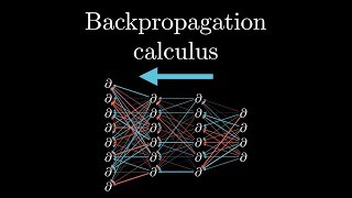Backprop intuitively3Blue1Brown · Backprop intuition visually explained

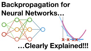Backprop calculus3Blue1Brown · Chain rule math formal

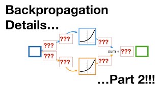Backprop Main IdeasStatQuest · Backprop overview optimization intro

Backprop Chain RuleStatQuest · Chain rule full optimization

Training with backpropagation Search on YouTube

Training finds the best learnable parameters of a network. It repeats three steps: feedforward, loss calculation, and backpropagation. Each cycle nudges every weight and bias. Many cycles drive the loss down.

Feedforward alone only predicts. The loss scores the prediction against the label. Backpropagation assigns credit to each weight for that score. Without this loop the network cannot learn.

Feed, Loss, Push: F-L-P

Feedforward sends inputs forward · Loss scores the prediction · Push gradients back and update each weight.

Feedforward pass Search on YouTube

Feedforward sends the input vector through the network layer by layer. Each neuron forms a weighted sum of its inputs plus a bias. Then it applies its activation function. The slides write the hidden output as $a = f(z)$ and pass it on as $h = a$ . They write the final output as $O = F(z)$ .

z = \sum_i w_i x_i + b \qquad a = f(z) \qquad h = a \qquad O = F(z)

$z$ = weighted sum plus bias at one neuron. $w_i$ = weight on input $x_i$ . $b$ = bias of the neuron. $f$ and $F$ = activation functions. $O$ = network output.

Hidden-layer sums Search on YouTube

The hidden layer converts raw inputs into learned features. Each hidden neuron has its own weights and bias. Its output becomes an input of the next layer.

Output-layer sum Search on YouTube

The output layer combines the hidden outputs into one sum. It adds its own bias and applies its own activation function. That result is the prediction $O$ .

The 2-2-1 network of the worked example. Each arrow carries a weight and each neuron adds a bias.

Worked example. Inputs $x_1 = 0.5$ and $x_2 = 0.3$ . Hidden neuron 1 uses weights $0.4$ and $0.2$ with bias $0.1$ . Hidden neuron 2 uses weights $0.3$ and $0.5$ with bias $-0.1$ . The output neuron uses weights $0.6$ and $0.4$ with bias $0.1$ . Every activation is the sigmoid $\sigma$ . The label is $y = 1$ .

Step 1. Hidden weighted sums.

\begin{aligned} z_{h1} &= 0.4(0.5) + 0.2(0.3) + 0.1 = 0.36\\ z_{h2} &= 0.3(0.5) + 0.5(0.3) - 0.1 = 0.20 \end{aligned}

Step 2. Hidden activations. Apply $\sigma(z) = 1/(1+e^{-z})$ .

\begin{aligned} h_1 &= \sigma(0.36) = 0.5890\\ h_2 &= \sigma(0.20) = 0.5498 \end{aligned}

Step 3. Output sum and prediction.

\begin{aligned} z_o &= 0.6(0.5890) + 0.4(0.5498) + 0.1 = 0.6734\\ O &= \sigma(0.6734) = \mathbf{0.6623} \end{aligned}

Loss calculation Search on YouTube

Loss measures the gap between the prediction and the label for one sample. The slides use the mean squared error (MSE). With one sample ( $n = 1$ ) the mean is the single squared gap.

L(y, O) = \frac{1}{n}\sum_{i=1}^{n}(y_i - O_i)^2

$y_i$ = label of sample $i$ . $O_i$ = network prediction for sample $i$ . $n$ = number of samples. Square the gap so positive and negative gaps both add cost.

Worked example. The network above predicts $O = 0.6623$ for label $y = 1$ ( $n = 1$ ).

\begin{aligned} L &= (1 - 0.6623)^2\\ &= (0.3377)^2\\ &= \mathbf{0.1141} \end{aligned}

Worked example. Two samples. Labels $1$ and $0$ . Predictions $0.7$ and $0.3$ .

\begin{aligned} L_1 &= (1 - 0.7)^2 = 0.09\\ L_2 &= (0 - 0.3)^2 = 0.09\\ L &= (0.09 + 0.09)/2 = \mathbf{0.09} \end{aligned}

Backpropagation at the output layer Search on YouTube

Backpropagation sends the loss signal backward through the network. The chain rule splits each gradient into a product of local partials. The output layer comes first because it sits next to the loss.

\sigma^{\prime}(z) = \sigma(z)(1 - \sigma(z))

The slides call this Equation (1). It gives the slope of the sigmoid at any sum $z$ . Every sigmoid partial below uses it.

\delta_o = \frac{\partial L}{\partial z_o} = -2(y - O)\,O(1 - O) \qquad w := w - \eta\,\frac{\partial L}{\partial w}

$\delta_o$ = loss signal at the output sum. $\eta$ = learning rate (here $\eta = 0.1$ ). Each weight moves against its gradient. The bias updates the same way.

Worked example. Loss $L = 0.1141$ , $O = 0.6623$ , $y = 1$ , $\eta = 0.1$ .

Step 1. Output loss signal.

\begin{aligned} \frac{\partial L}{\partial O} &= -2(1 - 0.6623) = -0.6755\\ \frac{\partial O}{\partial z_o} &= 0.6623(1 - 0.6623) = 0.2237\\ \delta_o &= -0.6755 \times 0.2237 = \mathbf{-0.1511} \end{aligned}

Step 2. Output-layer gradients. Each gradient is the signal times its input.

\begin{aligned} \frac{\partial L}{\partial v_1} &= \delta_o h_1 = -0.1511 \times 0.5890 = -0.0890\\ \frac{\partial L}{\partial v_2} &= \delta_o h_2 = -0.1511 \times 0.5498 = -0.0831\\ \frac{\partial L}{\partial c} &= \delta_o = -0.1511 \end{aligned}

Step 3. Update with $\eta = 0.1$ . Subtract the learning rate times each gradient.

\begin{aligned} v_1 &:= 0.6 - 0.1(-0.0890) = \mathbf{0.6089}\\ v_2 &:= 0.4 - 0.1(-0.0831) = \mathbf{0.4083}\\ c &:= 0.1 - 0.1(-0.1511) = \mathbf{0.1151} \end{aligned}

Keep the sign. A negative gradient raises the weight because minus times minus is plus. Check the sign of $\delta_o$ before every update.

Backpropagation at the hidden layer Search on YouTube

The hidden layer needs the signal that passes through the output weights. Each hidden neuron gets only its share of $\delta_o$ . Then the sigmoid slope at its own sum shapes that share.

\delta_{h1} = \delta_o\,v_1\,h_1(1 - h_1) \qquad \delta_{h2} = \delta_o\,v_2\,h_2(1 - h_2)

$\delta_{h}$ = loss signal at a hidden sum. $v$ = output-layer weight on that hidden output. $h(1-h)$ = sigmoid slope from Equation (1). Hidden weights update with $w := w - \eta\,\delta_h x$ .

Worked example. Signal $\delta_o = -0.1511$ flows back through $v_1 = 0.6$ and $v_2 = 0.4$ .

Step 1. Hidden loss signals.

\begin{aligned} \delta_{h1} &= -0.1511 \times 0.6 \times 0.5890 \times 0.4110 = \mathbf{-0.0219}\\ \delta_{h2} &= -0.1511 \times 0.4 \times 0.5498 \times 0.4502 = \mathbf{-0.0150} \end{aligned}

Step 2. Hidden gradients. Multiply each signal by its input ( $x_1 = 0.5$ , $x_2 = 0.3$ ).

\begin{aligned} \partial L/\partial w_{11} &= -0.0219 \times 0.5 = -0.0110\\ \partial L/\partial w_{21} &= -0.0219 \times 0.3 = -0.0066\\ \partial L/\partial w_{12} &= -0.0150 \times 0.5 = -0.0075\\ \partial L/\partial w_{22} &= -0.0150 \times 0.3 = -0.0045 \end{aligned}

Step 3. Update with $\eta = 0.1$ .

\begin{aligned} w_{11} &:= 0.4 - 0.1(-0.0110) = \mathbf{0.4011}\\ w_{21} &:= 0.2 - 0.1(-0.0066) = \mathbf{0.2007}\\ b_1 &:= 0.1 - 0.1(-0.0219) = \mathbf{0.1022}\\ w_{12} &:= 0.3 - 0.1(-0.0075) = \mathbf{0.3007}\\ w_{22} &:= 0.5 - 0.1(-0.0045) = \mathbf{0.5004}\\ b_2 &:= -0.1 - 0.1(-0.0150) = \mathbf{-0.0985} \end{aligned}

Update the biases too. Students often update the weights and leave the biases fixed. The bias gradient equals the neuron signal, so its step is $\eta\,\delta$ .

Second feedforward pass Search on YouTube

One update ends one training round. A fresh feedforward pass with the new weights tests the round. The loss should fall.

Worked example. Use all six updated weights and both updated biases.

Step 1. New hidden outputs.

\begin{aligned} z_{h1} &= 0.4011(0.5) + 0.2007(0.3) + 0.1022 = 0.3629\\ h_1 &= \sigma(0.3629) = 0.5898\\ z_{h2} &= 0.3007(0.5) + 0.5004(0.3) - 0.0985 = 0.2020\\ h_2 &= \sigma(0.2020) = 0.5503 \end{aligned}

Step 2. New prediction and loss.

\begin{aligned} z_o &= 0.6089(0.5898) + 0.4083(0.5503) + 0.1151 = 0.6989\\ O &= \sigma(0.6989) = 0.6679\\ L &= (1 - 0.6679)^2 = \mathbf{0.1103} \end{aligned}

Step 3. Compare. Loss falls from $0.1141$ to $\mathbf{0.1103}$ . The update helps. Many more rounds follow.

The lab below replays the worked example on this page. It moves the loss signal back and updates each weight once.

The 2-2-1 network learns one sample with label 1. Circles hold activations and arrows hold weights.

Learning rate η = 0.10

Feedforward gives O = 0.6623 and loss L = 0.1141. Select a circle or an arrow. Run plays one update with learning rate 0.1.

Batch, SGD, and minibatch Search on YouTube

The update rule needs gradients, but the data size sets how often updates happen. Three schemes split the same epoch in different ways. One epoch means one full pass over the training set.

Method	Samples per update	Updates per epoch	Character
Batch GD	all $n$	$1$	stable gradient, slow per step
SGD	$1$	$n$	noisy steps, fast and frequent
Minibatch	$B$ ( $1 \lt B \lt n$ )	$n/B$	middle ground, used in practice

Batch GD sums the gradient over every sample before one step. SGD updates after each single sample. Minibatch updates after each small group of $B$ samples. Minibatch keeps some noise but stays efficient on modern hardware. The slides name all three as ways to minimize empirical risk.

Chain-rule equations Search on YouTube

The chain rule links the loss to any weight through the sums between them. Each factor is a local slope. Their product is the full gradient.

\frac{\partial L}{\partial w} = \frac{\partial L}{\partial O}\,\frac{\partial O}{\partial z}\,\frac{\partial z}{\partial w} \qquad \frac{\partial z}{\partial w} = x

$\partial L/\partial O$ = loss slope at the prediction. $\partial O/\partial z$ = activation slope (use Equation (1) for sigmoid). $\partial z/\partial w$ = the input $x$ that the weight scales. Deeper weights chain more factors.

Empirical risk minimization Search on YouTube

Training minimizes the average loss on the training set. This average has a name: empirical risk. The theory behind it starts with the data distribution.

Joint data distribution Search on YouTube

Supervised data holds pairs $(X, y)$ . Here $X$ is an input feature vector and $y$ is its label. A joint probability distribution $P(X, y)$ governs how these pairs arise. It states the chance of each input and label happening together. It acts like the real-world rule that produces labels for inputs.

The true distribution stays unknown. The training set is only a finite sample drawn from it. The goal is a function $f_{\theta}$ that mimics the true map from $X$ to $y$ . Here $\theta$ is the parameter vector holding all weights and biases. A good $f_{\theta}$ works on new samples, not only on training samples.

Empirical risk Search on YouTube

R(\theta) = \frac{1}{n}\sum_{i=1}^{n}L(y_i, f(X_i, \theta))

$R(\theta)$ = empirical risk for parameters $\theta$ . $L$ = per-sample loss. $f(X_i, \theta)$ = prediction, which depends on both the input vector and the parameters. Empirical risk is the average loss over all training samples. Training minimizes it with gradient descent, SGD, or momentum methods.

Worked example. Four samples give losses $0.04$ , $0.09$ , $0.16$ , and $0.25$ .

\begin{aligned} R &= (0.04 + 0.09 + 0.16 + 0.25)/4\\ &= 0.54/4\\ &= \mathbf{0.135} \end{aligned}

The single number $0.135$ scores the whole training set. The optimizer drives it down step by step.

Do not trust a low training loss alone. A model can memorize training samples yet fail on new data. Low empirical risk must still generalize to the true distribution.

Quick self-test Search on YouTube

1. Name the three training steps in order.

Feedforward, loss calculation, backpropagation. Repeat the three to lower the loss.

2. Inputs are 0.5 and 0.3. A neuron has weights 0.4 and 0.2 with bias 0.1. Find z and h with a sigmoid.

$z = 0.4(0.5) + 0.2(0.3) + 0.1 = 0.36$ . $h = \sigma(0.36) = 0.5890$ .

3. Label is 1 and prediction is 0.6623. Find the MSE loss for n = 1.

$L = (1 - 0.6623)^2 = 0.1141$ . One sample means the mean equals the single squared gap.

4. Given output signal -0.1511 and hidden output 0.5890, find the gradient for their connecting weight.

Multiply signal by input: $-0.1511 \times 0.5890 = -0.0890$ . With $\eta = 0.1$ the weight rises by $0.0089$ .

5. Why does the hidden signal multiply by h(1 - h)?

$h(1-h)$ is the sigmoid slope from Equation (1). It converts the signal at the hidden output into a signal at the hidden sum.

6. Differentiate batch GD, SGD, and minibatch by updates per epoch.

Batch GD makes $1$ update per epoch. SGD makes $n$ updates. Minibatch makes $n/B$ updates. Minibatch is the practical middle ground.

7. A weight is 0.4 and its gradient is -0.0110. Update it with learning rate 0.1.

$w := 0.4 - 0.1(-0.0110) = 0.4011$ . The negative gradient raises the weight.

8. Four losses are 0.04, 0.09, 0.16, 0.25. Find the empirical risk.

$R = 0.54/4 = 0.135$ . Empirical risk is the average loss over training samples.

9. After one update the loss falls from 0.1141 to 0.1103. Does training stop now?

No. One step only starts the process. Training repeats feedforward, loss, and backpropagation until the loss settles.

10. Training loss is near zero but new data scores poorly. What went wrong?

The model fits training samples without matching the true distribution. Low empirical risk alone does not guarantee new-data results.

Training repeats three steps: feedforward, loss calculation, backpropagation.
Feedforward builds $z = \sum w_i x_i + b$ , then $a = f(z)$ with $h = a$ , and $O = F(z)$ .
MSE loss is $L = (1/n)\sum (y_i - O_i)^2$ ; the example gives $0.1141$ .
Sigmoid slope (Equation 1) is $\sigma^{\prime}(z) = \sigma(z)(1-\sigma(z))$ .
Output signal is $\delta_o = -2(y-O)O(1-O)$ ; weights move by $w := w - \eta\,\partial L/\partial w$ with $\eta = 0.1$ .
Hidden signals are $\delta_h = \delta_o v h(1-h)$ ; biases update too.
The second feedforward pass cuts the loss from $0.1141$ to $0.1103$ .
Batch GD uses all $n$ samples per update, SGD uses $1$ , minibatch uses $B$ .
Empirical risk is $R(\theta) = (1/n)\sum L(y_i, f(X_i, \theta))$ ; the example gives $0.135$ .
Low training loss alone does not guarantee good results on new data.

Backpropagation & empirical risk

Training with backpropagationSearch on YouTubeBookmarkSaved

Feedforward passSearch on YouTubeBookmarkSaved

Hidden-layer sumsSearch on YouTubeBookmarkSaved

Output-layer sumSearch on YouTubeBookmarkSaved

Loss calculationSearch on YouTubeBookmarkSaved

Backpropagation at the output layerSearch on YouTubeBookmarkSaved

Backpropagation at the hidden layerSearch on YouTubeBookmarkSaved

Second feedforward passSearch on YouTubeBookmarkSaved

Batch, SGD, and minibatchSearch on YouTubeBookmarkSaved

Chain-rule equationsSearch on YouTubeBookmarkSaved

Empirical risk minimizationSearch on YouTubeBookmarkSaved

Joint data distributionSearch on YouTubeBookmarkSaved

Empirical riskSearch on YouTubeBookmarkSaved

Quick self-testSearch on YouTubeBookmarkSaved

On this page