LSTM, GRU and bidirectional RNN
This lecture fixes the memory problem of plain RNNs with gated cells (LSTM, GRU). It then reads sequences in both directions (Bi-LSTM, Bi-RNN). After this page you can compute gate outputs, GRU updates, merge shapes and embedding lookups by hand.
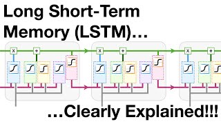 LSTM Clearly Explained
 Illustrated LSTM GRU Guide
 Seq2Seq Encoder-Decoder
Why long sequences break plain RNNsSearch on YouTube
A plain RNN keeps one hidden state. It rewrites this state at each step with the new input. Old information gets morphed at each step. After many steps the first inputs leave almost no trace.
The slides show this with a short gap. The sky is blank. The answer is blue. A short context is enough. A plain RNN predicts this well.
The slides then show a long gap. Harit lives in India for 13 years. He loves movies and works as an artist. He is very fluent in blank. The answer is Hindi. The clue (India) sits far from the blank. A plain RNN struggles here. It has morphed the early clue away.
The slides show a subject switch. Mark is a good singer and lived in LA for three years. Jacob is also a good singer. His debut was a great success. Congrats blank. The answer is Jacob. The model must forget Mark and keep Jacob. A plain RNN has no clear forget path.
LSTM is a notebook with an eraser and a gate. The cell keeps old notes. The gates erase stale notes and add fresh notes. The reader sees only a clean copy.
Cell state and hidden stateSearch on YouTube
An RNN has one vector: the hidden state . It stores memory and it also drives the output. These two roles clash. Storage needs stability. Output needs change.
LSTM splits the roles into two vectors. The cell state stores information (internal memory). The hidden state produces the output and prediction. Gates control the flow between them.
- Cell state : a slow conveyor. It carries facts across many steps. Changes to it are small and gated.
- Hidden state : a filtered view of . It feeds the classifier and the next step.
LSTM gatesSearch on YouTube
LSTM uses three gates. Each gate is a sigmoid in . A value blocks flow. A value passes all flow.
The three gates act in order. The forget gate drops stale memory. The input gate adds fresh memory. The output gate filters what leaves.
F-I-O: Forget past, Input new, Output filtered
Forget drops part of · Input adds the candidate to · Output filters into .
Shapes and batch-first layoutSearch on YouTube
The slides use for batch size (number of words in the batch). They use for feature size (size of each word vector). They use for hidden size (number of hidden units).
In batch-first layout each input batch has shape . Here is sequence length. Each hidden and cell state has shape . A matrix maps input to hidden. A matrix maps hidden to hidden. A result holds one row per sequence.
Practical frameworks favour batch-first layout. Without batching each vector is a column. With batching each vector is a row block.
Forget gateSearch on YouTube
The forget gate decides which part of to keep. It reads and . It outputs in .
is (input to gate). is (hidden to gate). is the bias of size . is sigmoid. has shape .
A value near keeps the old cell entry. A value near erases it. For the Mark-Jacob story the gate learns to erase Mark when Jacob arrives.
Input gate and candidateSearch on YouTube
The input gate has two parts. The gate decides where to write. The candidate holds the new values. The value stores nothing. The value stores the full candidate.
is and is . The output has shape .
is and is . The candidate lies in .
is element-wise product. has shape .
The cell update is a sum. The old term keeps gated memory. The new term adds gated input. This sum path carries gradients far. It avoids the fast decay of plain RNNs.
Output gate and hidden stateSearch on YouTube
The output gate decides which part of to show. A closed gate () blocks the cell. An open gate () passes all of it.
is and is . The output has shape .
has shape . The bounds the cell to before filtering.
The slides stress two computation styles. Separate computation learns one matrix per gate. Unified computation stacks the four matrices and learns once. Both learn the same count of parameters. Unified form runs faster.
Worked example. One cell unit. Prior cell . Pre-activation sums are , , , .
Gates. Apply sigmoid and .
Cell and hidden state. Combine old memory and new input.
The cell keeps most of the past (0.24) and adds some present (0.19). The output gate then passes 69 percent of it.
Exam shortcut: sigmoid gives and large positive gives near . gives . Test , first. Then (pure memory).
Move the gate sliders and watch the cell state update. The readout repeats the lecture numbers at each step.
Valve shade shows gate value. A shut valve blocks flow.
C = 0.5987 x 0.4 + 0.4013 x 0.4621 = 0.2395 + 0.1854 = 0.4249; h = 0.6900 x tanh(0.4249) = 0.2767
GRUSearch on YouTube
LSTM trains slowly. It learns four gate matrices per step. GRU is a simpler LSTM with two gates and one state. It merges cell and hidden state into one hidden state . It is faster and uses fewer parameters.
GRU gates:
- Reset gate : controls how much of enters the candidate.
- Update gate : decides how much of the candidate replaces .
has shape . A value near ignores the past when forming the candidate.
has shape . A value near takes the new candidate. A value near keeps the old state.
The reset gate sits inside the candidate. It scales before the matrix acts.
has shape . The two weights sum to per unit.
The last line can copy the past directly. When is near , stays near . This direct copy path cuts the vanishing effect.
Worked example. One GRU unit. Prior state . Pre-activation sums are , , .
Gates and candidate.
Final state. Mix past and candidate with weights that sum to .
The update gate keeps 40 percent of the past and takes 60 percent of the candidate.
| LSTM | GRU |
|---|---|
| Two states ( and ) | One state () |
| Three gates (forget, input, output) | Two gates (reset, update) |
| Four plus four matrices | Three of each |
| Slower training, strong on long gaps | Faster training, close accuracy on short gaps |
Bidirectional LSTMSearch on YouTube
A plain LSTM reads past and present only. State at time sees . Some tasks need the future too. A missing word may depend on words after it.
The slides show fill-in (interpolation). I am blank. Add one clue: I am blank hungry. Add more: I am blank hungry, I can eat a whole pig. Each future word narrows the blank. One direction alone cannot use the later words.
The slides show NER with apple. Sentence A: Dhaval loves apple, it keeps him healthy. Here apple is fruit. Sentence B: Dhaval loves apple, he bought their latest phone. Here apple is a brand. The word after apple (it versus he, healthy versus phone) fixes the label. A forward-only reader tags too early.
Bi-LSTM fixes this. It runs two LSTM layers. One reads forward from step to . One reads backward from step to . Each layer keeps its own hidden and cell states. At each step it combines the two hidden states.
Forward passSearch on YouTube
The forward LSTM reads first and last. At step it uses , forward and forward . It stores past context.
Backward passSearch on YouTube
The backward LSTM reads first and last. At step it uses , backward and backward . It stores future context.
Combine stepSearch on YouTube
After both passes each step has two vectors. The model merges them into one output.
is the forward hidden state of size . is the backward hidden state of size . is concat. has size .
maps to the label size. Other merges (sum, average, max) keep size .
Benefits and drawbacksSearch on YouTube
Benefits:
- It sees past and future context at each step.
- It captures long-range ties in both directions.
- It scores higher on speech, translation and sentiment tasks.
- It accepts extra layers such as attention on top.
Drawbacks:
- It costs about twice the compute of one LSTM.
- It needs large data to avoid overfitting.
- It is hard to interpret (a black box).
WorkflowSearch on YouTube
- Take the input sequence (words or characters as vectors).
- Map tokens to dense embeddings (semantic vectors).
- Run the Bi-LSTM layer over past and future context.
- Combine forward and backward states at each step (concat or transform).
Worked example. Batch , length , hidden size per direction. Each direction output has shape .
Concat merge. Stack the last axis.
Sum, average and max merges. Keep the same shape.
Concat doubles the classifier input. The other three keep it at .
Bidirectional RNNSearch on YouTube
A Bi-RNN applies the same two-direction idea with plain RNN cells. It passes the input through two RNNs. One reads forward and one reads in reverse. It then merges the two outputs into one final output.
Bi-RNN suits NLP and speech tasks. Plain RNN suits time-series prediction. Time series has no future at test time. Text tagging can use both sides.
Dual BPTTSearch on YouTube
Training uses two backprop passes. The forward RNN reads the sequence in order. Its error updates the forward weights. The backward RNN reads the sequence in reverse. Its error updates the backward weights. The loop repeats until the model converges. Both sides then shape each prediction.
Merge modesSearch on YouTube
The slides list four merges. The choice depends on the task. Concat is the default. It works well in many cases.
Concat stacks the two vectors. An output has size .
Sum adds the vectors element-wise. The shape stays .
Average means the element-wise mean. The shape stays .
Maximum takes the larger entry per unit. The shape stays .
C-S-A-M: Concat, Sum, Average, Max
Concat doubles size () · Sum adds · Average halves the sum · Max picks the larger entry.
Do not use Bi-RNN for live forecasting. Future inputs do not exist at test time. Use a forward-only RNN or LSTM there.
Text to vectorsSearch on YouTube
A network needs numbers, not letters. The pipeline turns text into vectors. It has four stages: text, tokenize, token IDs and embedding lookup. Each word then enters the net as an -dim vector at time .
- Split text into tokens (words or sub-words).
- Map each token to an integer ID from the vocabulary.
- Look up each ID in the embedding matrix (one row per token).
- Feed the -dim rows in order (pad short sentences to equal length).
One-hot form is (one in a long sparse row). The embedding matrix is (one dense row per word). Lookup skips the sparse product. It copies rows by index. This cuts sparse compute.
Vector options:
- One-hot: a sparse vector per token.
- Bag of words: counts per word (order lost).
- TF-IDF: counts weighted by rarity across docs.
- Word embeddings: dense vectors (Word2Vec, GloVe, FastText).
- Contextual embeddings: vectors that shift with context (BERT, RoBERTa).
Static versus contextual embeddingsSearch on YouTube
Static vectors give one vector per word. The slides use bank. Sentence 1: The bank approved my loan. Sentence 2: I sat on the bank of the river. The static vector is about in both. It cannot shift sense.
Contextual models read the full context (e.g. with a Transformer). The same word then gets two vectors. Loan-bank gives about . River-bank gives about . The vectors differ. The model can tag finance versus nature.
Worked example. Use the three shown entries of each bank vector. Static vectors are equal, so their gap is zero. Contextual vectors differ.
The static gap is . The contextual gap is . The shift separates the two senses.
Embedding matrix, OOV and fine-tuneSearch on YouTube
Two ways to get the matrix:
- Train it with the task (random start, learn rows with the model).
- Use pretrained rows (Word2Vec, GloVe, FastText).
Out-of-vocabulary (OOV) words miss the table. Two fixes exist. Map them to one unknown vector. Or build them from sub-word parts (FastText style).
Fine-tune means keep training the rows on task data. Do not train a fresh Word2Vec only on new words. Its space can sit in a new coordinate frame. Then old and new rows clash. Train jointly or learn a map between spaces.
Exam phrasing: static embeddings map one word to one vector; contextual embeddings map one word plus context to one vector. Name Word2Vec/GloVe for static and BERT for contextual.
Quick self-testSearch on YouTube
1. Why does a plain RNN fail on the Harit-Hindi sentence?
It rewrites one state at each step. The early clue (India) fades over the long gap. LSTM keeps it on the cell path.
2. State the roles of cell state and hidden state in one line each.
Cell state stores facts across steps. Hidden state is the filtered output shown to the next layer.
3. Pre-activations are 0.4 (forget), -0.4 (input), 0.5 (candidate), 0.8 (output), with prior cell 0.4. Find the new cell and hidden state.
, , candidate , . and .
4. Differentiate reset gate and update gate of a GRU.
Reset scales the past inside the candidate. Update mixes the candidate with the past. Small keeps .
5. GRU has prior state 0.6, reset pre-activation -0.2, update pre-activation 0.4 and candidate 0.1974. Find the new state.
and . .
6. Why does the apple NER case need a backward pass?
The label of apple depends on later words (it/healthy versus he/phone). A forward-only pass tags before it sees them.
7. Each Bi-LSTM direction gives shape (32, 10, 64). Give concat, sum, average and max shapes.
Concat gives . Sum, average and max each give .
8. List the four Bi-RNN merge modes and state which one changes the size.
Concat, sum, average and max. Only concat changes size ( to ). The rest keep .
9. Static bank vectors match in both sentences but contextual ones differ by 1.11 on the shown prefix. What does this show?
Static form stores one sense per word (gap 0). Contextual form stores sense plus context (gap 1.11). Hence river-bank and loan-bank split.
10. How do you handle OOV words, and what is wrong with a separate Word2Vec only for new words?
Map OOV words to an unknown vector or build them from sub-words. A separate Word2Vec can land in a new coordinate frame. Then its rows clash with the old space.
- Plain RNNs morph old inputs away; long gaps (Harit-Hindi) and subject switches (Mark-Jacob) need gated memory.
- LSTM splits memory () from output (); gates are sigmoids in , candidate uses .
- Forget gate: ; input gate plus candidate build ; output gate gives .
- Shapes: input , states , maps and ; frameworks use batch-first layout.
- GRU merges states: reset , update , candidate , mix .
- Bi-LSTM runs forward and backward LSTMs and merges per step; it resolves fill-in blanks and apple NER via future words.
- Bi-RNN runs two RNNs with dual BPTT; merges are concat (), sum, average and max (each ).
- Text pipeline: tokenize, map to IDs, look up rows, feed -dim vectors; static bank vectors match while contextual loan/river vectors differ.
- OOV fix: unknown vector or sub-word parts; fine-tune jointly so spaces stay aligned.