ANN blocks and activations

This lecture names the building blocks of a neural network (neuron, input layer, hidden layer, output layer). It shows how connections, learning rules and activation functions describe any model. After this page you can compute activation outputs and softmax probabilities by hand. You can also pair each task with the right output-layer activation.

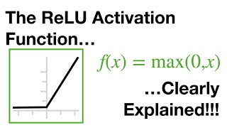But what is a neural network?3Blue1Brown · Neuron layers intro visual

ReLU In ActionStatQuest · ReLU activation deep nets

ArgMax and SoftMaxStatQuest · Softmax multi-class outputs

Activation Functions VisuallyVector Shield · Sigmoid ReLU softmax overview

Why networks need non-linearity Search on YouTube

A single-layer network draws only straight boundaries. It cannot capture non-linear functions. Higher variants of the network add hidden layers and non-linear activation functions. Those variants learn curves and complex regions.

Components of an ANN Search on YouTube

An ANN has four building blocks. They are the neuron, the input layer, the hidden layer and the output layer. Each block has one clear job.

Neuron Search on YouTube

A neuron is a cell inside the ANN. It receives values and performs a computation. It holds the result $a$ , which shows the activation level of that neuron. The computation is a weighted sum of the inputs plus a bias value. The bias decides whether the neuron turns active.

z = \sum_{i=1}^{m} w_i x_i + b \qquad a = f(z)

$z$ is the weighted sum plus bias. $w_i$ are weights and $x_i$ are inputs. $b$ is the bias. $f$ is the activation function. $a$ is the activation level held by the neuron.

One neuron. Inputs meet weights, the bias joins the sum, and f sets the activation level.

Worked example. One neuron has weights $w = (0.5, -0.4, 0.3)$ and bias $b = 0.1$ . The input vector is $x = (2.0, 1.0, -1.0)$ .

Step 1. Weighted sum.

\begin{aligned} z &= 0.5(2.0) + (-0.4)(1.0) + 0.3(-1.0) + 0.1\\ &= 1.0 - 0.4 - 0.3 + 0.1 = \mathbf{0.4} \end{aligned}

Step 2. Activation outputs. ReLU keeps positives, so $\text{ReLU}(0.4) = \mathbf{0.4}$ . The sigmoid gives $\sigma(0.4) = 1/(1+e^{-0.4}) = 1/1.6703 = \mathbf{0.599}$ . The same $z$ gives different answers under different activation functions.

Input layer Search on YouTube

The input layer is the first layer of the ANN. It receives the direct input, a set of values used for computation. An input with $m$ dimensions is an input vector with $m$ dimensions.

In theory each input neuron is a placeholder for one dimension. It performs no computation. So the neuron count equals the dimension count. For $I_1 = \{x_{11}, x_{12}, x_{13}\}$ the input layer holds three neurons.

First dense layer in practice Search on YouTube

Libraries such as Keras design the first layer as a dense layer. Each neuron there receives a full copy of the whole input vector. So the neuron count need not equal the input dimension count. A 3-dimensional input can feed a first dense layer with 16 neurons.

Hidden layer Search on YouTube

Hidden layers sit between the input layer and the output layer. Each hidden layer holds its own set of neurons, and counts vary across layers. Their job is to find patterns for each input and pass an output onward. Hidden layers give the network its non-linear power.

Output layer Search on YouTube

The output layer is the last layer in the ANN. It reads the values from the previous layer. It returns one or more values as the answer.

Basic architecture of an ANN Search on YouTube

The arrangement of neurons into layers is the network architecture. The connection pattern within and between layers is part of it too. Two networks with the same neurons but different wiring are different architectures.

Three aspects of an ANN Search on YouTube

Models differ along three aspects:

The synaptic interconnections of the model.
The training or learning rules that update the connection weights.
The activation functions of the neurons.

The next three sections follow this order.

Interconnections Search on YouTube

Interconnections fall into two types: feedforward and feedback. Feedforward sends data forward only. Feedback sends outputs back as inputs.

Feedforward moves X to H to Y with no return path. Feedback loops the output back.

Feedforward neural networks Search on YouTube

Data flows only one way: from input to hidden layers to output. No cycles or loops exist. Information moves forward. The Sequential model with Dense layers is one example. It suits classification and regression with fixed-size inputs.

model = Sequential([Dense(16, activation="relu"), Dense(10, activation="softmax")])

Single-layer perceptron Search on YouTube

A single-layer perceptron has no hidden layers. One input layer feeds the output layer directly. The output layer can hold one or more perceptrons. Each perceptron produces its own output, which suits multi-class classification. Each output neuron acts like a linear perceptron.

Multilayer perceptron Search on YouTube

A multilayer perceptron (MLP) stacks multiple neuron layers. It includes hidden layers. It handles linear and non-linear functions.

Single-layer perceptron	Multilayer perceptron
No hidden layer	One or more hidden layers
Input layer feeds output directly	Signals pass through hidden layers
Only linear boundaries	Linear and non-linear functions
One output per perceptron	Each output neuron gives one value

Feedback neural networks Search on YouTube

A feedback network sends outputs back as inputs to the same layer or a previous layer. Feedback to the same layer is lateral feedback. Networks use it to model competition or cooperation between neurons. In competitive learning, strong neurons suppress weak ones through lateral inhibition.

Feedback networks are also called recurrent or dynamic networks. Two feedback types exist:

Self-feedback: the output feeds back into the same neuron.
Cross-neuron feedback: the output feeds other neurons in the same or previous layers. Lateral feedback is cross-neuron feedback restricted to the same layer.

Such networks suit systems that must stabilise or converge over time.

Do not confuse a feedback network with reinforcement learning. A feedback network is wiring: outputs loop back as inputs. Reinforcement learning is a learning model: rewards shape actions. The slides stress this difference.

Recurrent neural networks Search on YouTube

A recurrent neural network (RNN) is a feedback network for sequences. Loops carry information from previous time steps into current processing. RNNs suit time series, language, speech and any sequential data. Variants include LSTM, GRU and bidirectional RNNs.

Single neuron with feedback Search on YouTube

This network looks like a perceptron. It adds one extra input: the feedback from its own output.

Single layer with feedback Search on YouTube

This network looks like a single-layer perceptron with no hidden layer. It takes feedback from the output as one of its inputs.

Multi-layer with feedback Search on YouTube

This network looks like an MLP. The output feeds back to itself or to another neuron in the same layer. It can also feed nodes in the preceding layer. That wiring forms a multilayer recurrent network.

Learning rules Search on YouTube

Learning in an ANN follows three aspects: parameter learning, structure learning and the learning model. Each aspect answers a different question: which values change, which wiring changes and which feedback signal guides change.

Parameter learning Search on YouTube

Parameter learning tunes the weights and biases. These are the learnable parameters of the model. Backpropagation and optimizers perform the tuning. Optimizers include Adam, SGD and RMSprop. They minimise the loss function.

\theta \leftarrow \theta - \eta\,\frac{d\,\text{Loss}}{d\theta}

$\theta$ is the parameter vector (weights and biases). $\eta$ is the learning rate. The derivative sets the direction and size of each step.

Structure learning Search on YouTube

Structure learning changes the network itself to find the best architecture. Neural Architecture Search (NAS) uses search algorithms such as RL, evolutionary algorithms and gradients. Pruning is another approach: it removes or zeroes out less useful neurons. Structure learning tunes the hyperparameters of the network. Tools include AutoML, Google NAS and ENAS.

Learning models Search on YouTube

The learning model decides which machine-learning feedback the ANN uses. Three models exist: supervised, unsupervised and reinforcement learning.

Supervised learning Search on YouTube

The input is a vector $(x_1, x_2, \dots, x_n)$ plus a target label. Together they form a training pair. The model trains on both inputs and labels. It can assess its own learning from this data. Parameters update toward optimal performance. Problems are variants of classification or regression.

Unsupervised learning Search on YouTube

The input is a vector with no target label. Parameter updates use only the input vector. The model must find patterns and organise them as clusters. It updates through contrastive objectives, clustering objectives or reconstruction loss in autoencoders. Outputs stay internal and guide parameter updates. They are not shared externally as neuron inputs.

Reinforcement learning Search on YouTube

This learning grows stronger through rewards and punishments for each action. The input vector defines the current state of the model. The output is the action taken. Feedback arrives as a response to the action. The response updates the current state of the model. The goal is an optimal strategy that maximises the cumulative reward.

Supervised	Unsupervised	Reinforcement
Input vector plus label	Input vector only	State vector plus reward signal
Loss against labels	Clustering or reconstruction objectives	Cumulative reward objective
Classification or regression	Clusters and features	Optimal action strategy

Activation functions Search on YouTube

Activation functions introduce non-linearity into the network. Without them, stacked layers would collapse into one linear map. Weights and biases are the learnable parameters. Activation functions shape what those parameters express.

Think of a dimmer switch with different brands. Each brand maps the same knob position to its own brightness. The knob is $z$ . The brand is the activation function.

What an activation function does Search on YouTube

An activation function sets the neuron activity level from $z$ . Each function defines its own outcome for the same $z$ . For example, $\text{ReLU}(-1)$ equals 0 while $\sigma(-1)$ stays above 0. Hidden layers and the output layer usually use different activation functions. The problem at hand decides the output-layer choice.

Types of activation functions Search on YouTube

The slides name seven functions: identity (linear), step, sign, sigmoid (logistic), tanh (hyperbolic), ReLU and softmax.

\begin{aligned} \text{Identity:}\quad f(z) &= z\\ \text{Step:}\quad f(z) &= 0 \text{ if } z \lt 0,\; 1 \text{ if } z \ge 0\\ \text{Sign:}\quad f(z) &= -1 \text{ if } z \lt 0,\; 0 \text{ if } z = 0,\; +1 \text{ if } z \gt 0\\ \text{Sigmoid:}\quad \sigma(z) &= \frac{1}{1 + e^{-z}}\\ \text{Tanh:}\quad \tanh(z) &= \frac{e^{z} - e^{-z}}{e^{z} + e^{-z}}\\ \text{ReLU:}\quad f(z) &= \max(0, z)\\ \text{SiLU:}\quad f(z) &= z\,\sigma(z) \end{aligned}

Identity returns $z$ unchanged. Step returns a binary 0 or 1. Sign returns $-1$ , 0 or $+1$ . Sigmoid maps $z$ into $(0, 1)$ . Tanh maps $z$ into $(-1, 1)$ . ReLU zeroes negatives and keeps positives. SiLU multiplies $z$ by its own sigmoid.

Fix the step convention before the exam and state it. This page uses 0 for $z \lt 0$ and 1 for $z \ge 0$ . Some texts put 1 only for $z \gt 0$ . Examiners accept either convention when stated.

Worked example. Compute all six single-input activation outputs for $z = -1$ , $z = 0$ and $z = 2$ .

Step 1. Identity, step and sign.

\begin{aligned} \text{Identity:} &\quad -1,\; 0,\; 2\\ \text{Step:} &\quad 0,\; 1,\; 1 \quad (0 \text{ counts as active here})\\ \text{Sign:} &\quad -1,\; 0,\; +1 \end{aligned}

Step 2. Sigmoid. Use $\sigma(z) = 1/(1+e^{-z})$ .

\begin{aligned} \sigma(-1) &= 1/(1 + e) = 1/3.7183 = \mathbf{0.269}\\ \sigma(0) &= 1/2 = \mathbf{0.5}\\ \sigma(2) &= 1/(1 + e^{-2}) = 1/1.1353 = \mathbf{0.881} \end{aligned}

Step 3. Tanh and ReLU.

\begin{aligned} \tanh(-1) &= (1 - e^{2})/(1 + e^{2}) = -6.389/8.389 = \mathbf{-0.762}\\ \tanh(0) &= \mathbf{0}\\ \tanh(2) &= (e^{4}-1)/(e^{4}+1) = 53.598/55.598 = \mathbf{0.964}\\ \text{ReLU:} &\quad 0,\; 0,\; 2 \end{aligned}

Identity and ReLU match for $z \ge 0$ and differ for $z \lt 0$ . Sigmoid stays above 0 at $z = -1$ while ReLU gives exactly 0.

Softmax Search on YouTube

Softmax takes a vector $z = (z_1, z_2, \dots, z_k)$ and returns a vector of the same length. It converts arbitrary real values into a probability distribution. The probabilities sum to 1.

f_i(z_i) = \frac{\exp(z_i)}{\sum_{j=1}^{k}\exp(z_j)} \qquad \sum_{i=1}^{k} f_i = 1

$f_i$ is the probability of class $i$ . The numerator exponentiates one logit. The denominator sums exponentials over all $k$ classes.

Worked example. Logits are $z = (2.0, 1.0, 0.1)$ . Turn them into probabilities.

Step 1. Exponentiate each logit.

\begin{aligned} e^{2.0} &= 7.3891\\ e^{1.0} &= 2.7183\\ e^{0.1} &= 1.1052 \end{aligned}

Step 2. Sum and divide.

\begin{aligned} S &= 7.3891 + 2.7183 + 1.1052 = 11.2126\\ p_1 &= 7.3891/11.2126 = \mathbf{0.659}\\ p_2 &= 2.7183/11.2126 = \mathbf{0.242}\\ p_3 &= 1.1052/11.2126 = \mathbf{0.099} \end{aligned}

Step 3. Check. $0.659 + 0.242 + 0.099 = 1.000$ . Class 1 wins with probability 0.659.

Step 4. Stable repeat (extra check). Subtract the maximum 2.0 first: $(0, -1, -1.9)$ . Exponentials are 1, $0.3679$ and $0.1496$ . The sum is $1.5175$ . Then $p_1 = 1/1.5175 = \mathbf{0.659}$ . Shifting all logits leaves every probability unchanged.

Softmax is interdependent Search on YouTube

ReLU and sigmoid map one input to one output. Their graphs fit a flat 2D plane of $y = f(z)$ . Softmax is a multivariable function. Each class output depends on the exponential sum over all classes. Change one input number and every class probability shifts. The other inputs stay fixed, yet their shares still move.

Output-layer and hidden-layer rules Search on YouTube

The task decides the output activation. The network type suggests the hidden activation.

Task	Output activation	Reason
Regression	Linear (identity)	Outputs need any real value
Binary classification	Sigmoid	One output in $(0, 1)$
Multiclass classification	Softmax	Probabilities over classes sum to 1
Multi-label classification	Sigmoid per label	Each label gets its own probability; sums do NOT reach 1

Network	Hidden activation	Reason
Convolutional network	ReLU	Sparse and cheap activations
Recurrent network	Tanh or sigmoid	Bounded values suit loops

Worked example. Pair each task with its output activation.

House-price prediction. Prices are continuous values. Use a linear output. One neuron returns the price directly.

Spam detection. The mail is spam or not spam. Use one sigmoid neuron. Outputs near 1 mean spam.

Digit recognition (0 to 9). Each image holds exactly one digit. Use softmax over 10 neurons. The 10 probabilities sum to 1.

Photo tagging (cat, outdoor, night). One photo can carry several tags. Use one sigmoid neuron per tag. Each probability stands alone, so the three need not sum to 1.

I Step, I Sign, I Sigmoid, I Tanh, I Rectify, I Soften: I-S-S-S-T-R-S

Identity · Step · Sign · Sigmoid · Tanh · ReLU · Softmax. Seven functions in slide order.

Regression-Linear, Binary-Sigmoid, Multi-Softmax, Labels-Sigmoid: R-B-M-L

Regression uses Linear · Binary uses Sigmoid. Multiclass uses Softmax · multi-Label uses one Sigmoid per label. Hidden layers: CNN pairs with ReLU, RNN pairs with Tanh or sigmoid.

Differentiation of activation functions Search on YouTube

Backpropagation updates each weight and bias from the gradient of the loss. The chain rule passes through every activation function. So the differentiability of the activation function matters.

Three cases follow:

Zero derivative: the parameter does not change. Training gets stuck.
Very small derivative: the parameter changes too slowly. This is the vanishing gradient.
Very large derivative: the parameter may jump too far. This is the exploding gradient.

Key derivatives (extra)Search on YouTube

These standard results show why the three cases above occur.

\begin{aligned} \sigma'(z) &= \sigma(z)\,(1 - \sigma(z)) \le 0.25\\ \tanh'(z) &= 1 - \tanh^{2}(z)\\ \text{ReLU}'(z) &= 0 \text{ if } z \lt 0,\; 1 \text{ if } z \gt 0 \end{aligned}

Sigmoid slopes peak at 0.25, so deep stacks shrink gradients fast. Tanh slopes peak at 1. ReLU passes full gradient for positives and zero for negatives.

Worked example. Compare gradient flow at three operating points.

Step 1. Sigmoid at $z = 0$ . $\sigma(0) = 0.5$ . Slope $= 0.5 \times 0.5 = \mathbf{0.25}$ . This is the strongest sigmoid gradient.

Step 2. Sigmoid at $z = 5$ . $\sigma(5) = 148.413/149.413 = 0.9933$ . Slope $= 0.9933 \times 0.0067 = \mathbf{0.00665}$ . The neuron is saturated, so the parameter barely moves.

Step 3. ReLU at $z = 2$ and $z = -1$ . Slope $= \mathbf{1}$ at $z = 2$ . Slope $= \mathbf{0}$ at $z = -1$ . The negative input blocks learning through that neuron.

Step 4. Tanh at $z = 3$ . $\tanh(3) = 402.429/404.429 = 0.9951$ . Slope $= 1 - 0.9901 = \mathbf{0.0099}$ . Saturation strikes here too.

Step function vs sigmoid Search on YouTube

The slides contrast the step curve with the sigmoid curve. Step jumps from 0 to 1 at the threshold. Its slope is zero almost everywhere, so no gradient flows. Sigmoid smooths the same jump into an S-curve. Its slope stays nonzero, so learning proceeds. Differentiability is the practical difference between them.

ReLU Search on YouTube

ReLU means Rectified Linear Unit. It removes all negative outputs from the network. It joins two piece-wise linear parts, so the whole map stays non-linear. It allows sparse activations: many neurons output exact 0. Sparsity improves network efficiency. ReLU handles the vanishing gradient problem better than sigmoid and tanh. Positive inputs pass gradient 1, which never shrinks.

SiLU Search on YouTube

SiLU means Sigmoid Linear Unit. It multiplies $z$ by $\sigma(z)$ . It is non-monotonic: its output does not always rise with $z$ . Small negatives dip below zero before the curve climbs. Image classification networks use it often.

GeLU Search on YouTube

GeLU means Gaussian Error Linear Unit. It combines a linear unit with a non-linear tanh form. It maps negatives smoothly toward values near zero. It keeps strong positive outputs for positive inputs. NLP models use it widely, including BERT, transformers and GPT 2/3.

\text{GeLU}(z) \approx 0.5\,z\left(1 + \tanh\left(\sqrt{2/\pi}\,\left(z + 0.044715\,z^{3}\right)\right)\right)

$z$ is the input. The tanh term bends the line smoothly. Large positives pass through almost unchanged. Large negatives fade toward zero.

Quick self-test Search on YouTube

1. A neuron has weights (0.5, -0.4, 0.3), bias 0.1 and input (2.0, 1.0, -1.0). Find z, ReLU(z) and σ(z).

$z = 1.0 - 0.4 - 0.3 + 0.1 = 0.4$ . $\text{ReLU}(0.4) = 0.4$ . $\sigma(0.4) = 1/1.6703 = 0.599$ .

2. Compute ReLU(-1), σ(-1), tanh(-1), step(-1) and sign(-1).

$\text{ReLU}(-1) = 0$ . $\sigma(-1) = 0.269$ . $\tanh(-1) = -0.762$ . Step gives 0. Sign gives $-1$ .

3. Logits are (2.0, 1.0, 0.1). Find the three softmax probabilities and name the winner.

Exponentials are 7.3891, 2.7183 and 1.1052. The sum is 11.2126. Probabilities are 0.659, 0.242 and 0.099. Class 1 wins.

4. Why does shifting all logits by the same constant leave softmax unchanged?

Each numerator and the denominator gain the same factor $e^{c}$ . The factor cancels in every ratio. The worked example shifts by $-2.0$ and still gets 0.659.

5. Pair each task with its output activation: house prices, spam detection, digit 0-9, photo with several tags.

House prices use linear. Spam uses one sigmoid neuron. Digits use softmax over 10. Photo tags use one sigmoid neuron per tag, since sums need not reach 1.

6. Differentiate a single-layer perceptron from a multilayer perceptron.

A single-layer perceptron has no hidden layer and learns only linear boundaries. An MLP adds hidden layers and learns non-linear functions too.

7. Differentiate self-feedback from cross-neuron feedback. What is lateral feedback?

Self-feedback returns the output to the same neuron. Cross-neuron feedback sends it to other neurons in the same or previous layers. Lateral feedback is cross-neuron feedback within the same layer.

8. σ(5) ≈ 0.9933. Find the slope there and state the training effect.

Slope $= 0.9933 \times 0.0067 = 0.00665$ . The neuron is saturated. The parameter barely moves, so learning stalls (vanishing gradient).

9. Why does ReLU beat sigmoid on the vanishing gradient, and what is its own failure case?

Positive inputs pass slope 1, which never shrinks through depth. Its failure case is slope 0 for negatives: a stuck neuron stops learning.

A single layer learns only linear boundaries. Hidden layers plus non-linear activation functions capture non-linear functions.
A neuron forms $z = \sum w_i x_i + b$ and holds $a = f(z)$ . $z = 0.4$ gives ReLU $0.4$ and sigmoid $0.599$ .
The input layer receives the input vector. Theory uses one placeholder neuron per dimension. Keras dense layers may use any neuron count.
Hidden layers find patterns between input and output. The output layer returns the final values.
Interconnections split into feedforward (one way, no cycles) and feedback (outputs return as inputs). RNNs are feedback networks for sequences.
Learning splits into parameter learning (weights and biases via $\theta \leftarrow \theta - \eta\,d\text{Loss}/d\theta$ ), structure learning (NAS, pruning) and the learning model (supervised, unsupervised, reinforcement).
Seven activation functions: identity, step, sign, sigmoid, tanh, ReLU, softmax. Memory hook: I-S-S-S-T-R-S.
Softmax $f_i = \exp(z_i)/\sum_j \exp(z_j)$ gives probabilities that sum to 1. Logits $(2.0, 1.0, 0.1)$ give $(0.659, 0.242, 0.099)$ .
Output rules: regression uses linear, binary uses sigmoid, multiclass uses softmax, multi-label uses one sigmoid per label. Hidden rules: CNN uses ReLU, RNN uses tanh or sigmoid.
Zero derivative stalls learning, tiny derivatives vanish and huge derivatives explode. Sigmoid peaks at slope $0.25$ . SiLU serves images, GeLU serves NLP models.

ANN blocks and activations

Why networks need non-linearitySearch on YouTubeBookmarkSaved

Components of an ANNSearch on YouTubeBookmarkSaved

NeuronSearch on YouTubeBookmarkSaved

Input layerSearch on YouTubeBookmarkSaved

First dense layer in practiceSearch on YouTubeBookmarkSaved

Hidden layerSearch on YouTubeBookmarkSaved

Output layerSearch on YouTubeBookmarkSaved

Basic architecture of an ANNSearch on YouTubeBookmarkSaved

Three aspects of an ANNSearch on YouTubeBookmarkSaved

InterconnectionsSearch on YouTubeBookmarkSaved

Feedforward neural networksSearch on YouTubeBookmarkSaved

Single-layer perceptronSearch on YouTubeBookmarkSaved

Multilayer perceptronSearch on YouTubeBookmarkSaved

Feedback neural networksSearch on YouTubeBookmarkSaved

Recurrent neural networksSearch on YouTubeBookmarkSaved

Single neuron with feedbackSearch on YouTubeBookmarkSaved

Single layer with feedbackSearch on YouTubeBookmarkSaved

Multi-layer with feedbackSearch on YouTubeBookmarkSaved

Learning rulesSearch on YouTubeBookmarkSaved

Parameter learningSearch on YouTubeBookmarkSaved

Structure learningSearch on YouTubeBookmarkSaved

Learning modelsSearch on YouTubeBookmarkSaved

Supervised learningSearch on YouTubeBookmarkSaved

Unsupervised learningSearch on YouTubeBookmarkSaved

Reinforcement learningSearch on YouTubeBookmarkSaved

Activation functionsSearch on YouTubeBookmarkSaved

What an activation function doesSearch on YouTubeBookmarkSaved

Types of activation functionsSearch on YouTubeBookmarkSaved

SoftmaxSearch on YouTubeBookmarkSaved

Softmax is interdependentSearch on YouTubeBookmarkSaved

Output-layer and hidden-layer rulesSearch on YouTubeBookmarkSaved

Differentiation of activation functionsSearch on YouTubeBookmarkSaved

Key derivatives (extra)Search on YouTubeBookmarkSaved

Step function vs sigmoidSearch on YouTubeBookmarkSaved

ReLUSearch on YouTubeBookmarkSaved

SiLUSearch on YouTubeBookmarkSaved

GeLUSearch on YouTubeBookmarkSaved

Quick self-testSearch on YouTubeBookmarkSaved

On this page