Perceptron & linear separability

This lecture builds the perceptron from the biological neuron (MP neuron, Rosenblatt perceptron, step activation). It shows the decision boundary and linear separability with OR, AND and XOR. After this page you can run PLA updates on OR and solve thresholds for AND and OR.

But what is a neural network?3Blue1Brown · Neuron layers intro visual

Perceptron Explained VisuallyBeyond The Formula · PLA learning rule demo

Biological neuron to artificial neuron Search on YouTube

A biological neuron receives signals through dendrites. It processes them in the cell body. It fires through the axon when the net input passes a threshold. The hand-pulled-from-heat reflex shows this chain. Receptors sense heat, interneurons decide, motor neurons carry the response.

The artificial neuron copies this chain with numbers:

Artificial component	Biological part	Function
Inputs $x_1, x_2, \dots, x_n$	Dendrites	Receive signals
Weights $w_1, w_2, \dots, w_n$	Synaptic strength	Set signal importance
Sum $z$	Cell body (soma)	Combine inputs
Activation function $f(z)$	Firing mechanism	Decide output
Output $a$	Axon	Pass output onward

D-S-C-F-A

Dendrites take inputs · Synapses set weights · Cell body sums · Firing is activation · Axon sends output.

Computational units Search on YouTube

A computational unit is the basic building block of a neural network. It receives scalar inputs. It multiplies each input by a weight. It sums the products. It passes the sum through an activation function such as thresholding. It emits one output value.

Think of a voting panel. Each member casts a weighted vote. The chair adds the votes. The motion passes when the total crosses a fixed mark.

McCulloch-Pitts neuron Search on YouTube

McCulloch and Pitts published the MP neuron in 1943. It was one of the first formal neuron models. It performs binary logic with Boolean inputs. It has no learning. Its output follows a fixed threshold.

f(x) = \sum_{i=1}^{2} w_i x_i

$w_i$ are fixed weights. $x_i$ are Boolean inputs ( $0$ or $1$ ). The neuron fires when the sum reaches the threshold.

Threshold logic Search on YouTube

Threshold logic computes a function from a weighted sum. The neuron fires when the sum reaches a manually chosen threshold. No training adjusts the threshold. The designer picks it from the target logic.

Worked example: AND with an MP neuron. Set both weights to $1$ . Set the threshold to $2$ . The neuron fires only when both inputs are $1$ .

$x_1$	$x_2$	Sum $x_1 + x_2$	Output $a$
0	0	0	0
0	1	1	0
1	0	1	0
1	1	2	1

Check each row.

\begin{aligned} (0,0):\quad 0 &\lt 2 \;\Rightarrow\; \mathbf{0}\\ (0,1):\quad 1 &\lt 2 \;\Rightarrow\; \mathbf{0}\\ (1,0):\quad 1 &\lt 2 \;\Rightarrow\; \mathbf{0}\\ (1,1):\quad 2 &\ge 2 \;\Rightarrow\; \mathbf{1} \end{aligned}

The table matches AND. The threshold $2$ forces both inputs to be active.

a = \begin{cases} 1 & \text{if } \sum_{i=1}^{2} w_i x_i \ge 2\\ 0 & \text{if } \sum_{i=1}^{2} w_i x_i \lt 2 \end{cases}

$a$ is the output. The value $2$ is the fixed threshold for AND with unit weights.

MP neuron features Search on YouTube

Feature	Description
Inputs	Boolean ( $0$ or $1$ )
Weights	Fixed, typically positive integers
Sum	Adds the weighted inputs
Threshold	Fixed integer value
Activation function	Step: $1$ when sum $\ge$ threshold, else $0$
Output	Boolean ( $0$ or $1$ )
Learning	None (no weight updates)

Say "fixed threshold" for MP neurons in the exam. Say "learned weights and bias" for perceptrons. The contrast earns marks.

Supervised learning Search on YouTube

Supervised learning learns a mapping from inputs to outputs. The input vector is $X = [x_1, x_2, \dots, x_n]$ . The learning algorithm searches for a function $f$ . The model must fit the training data. It must also predict new records correctly.

\hat{y} = f(X)

$X$ is the attribute vector. $f$ is the learned function. $\hat{y}$ is the predicted output.

The slides show an $X \to Y$ table (for example $5 \to 27$ , $1 \to 3$ ). Each row pairs one input with its label. Learning means finding the $f$ behind such pairs.

Classification and regression Search on YouTube

Prediction learns a target function from each attribute set $x$ to an output $y$ . Classification predicts a categorical $y$ (spam or safe). Regression predicts a continuous $y$ (a number). The perceptron below does binary classification.

\text{loss} = Y - \hat{Y}

$Y$ is the true label. $\hat{Y}$ is the predicted output. The loss measures how wrong one prediction is.

Linear perceptron Search on YouTube

Rosenblatt proposed the perceptron in 1958. It is a single-neuron network. It was the first neuron model that could learn weights from data. It takes several inputs (real or Boolean). It applies weights and a bias. It passes the result through an activation function (typically a step). It handles only linear boundaries (a straight line or hyperplane).

The neuron output $a$ reports the activation level of that neuron. The slides call the activation function an "activity function" once. The canonical term is activation function.

Step and sigmoid activation Search on YouTube

The activation function decides the activity level of a neuron.

Step function Search on YouTube

The step uses a threshold $t$ (the bias form appears below). The neuron stays dormant below $t$ . It becomes active at and above $t$ .

Sigmoid Search on YouTube

The sigmoid gives graded activity between $0$ and $1$ . The same input sum can thus give many activity levels. The slides use four sample points.

a = \sigma(z) = \frac{1}{1 + e^{-z}}

$z$ is the weighted sum plus bias. $\sigma$ is the sigmoid. Large $z$ pushes $a$ toward $1$ . Small $z$ pushes $a$ toward $0$ .

Worked example: sigmoid activity levels. Apply $\sigma$ to the four slide inputs.

\begin{aligned} \sigma(-2.7) &= 1/(1 + e^{2.7}) = 1/15.88 = \mathbf{0.063}\\ \sigma(-0.9) &= 1/(1 + e^{0.9}) = 1/3.46 = \mathbf{0.289}\\ \sigma(0.7) &= 1/(1 + e^{-0.7}) = 1/1.497 = \mathbf{0.668}\\ \sigma(1.0) &= 1/(1 + e^{-1.0}) = 1/1.368 = \mathbf{0.731} \end{aligned}

Read the trend. Activity rises with $z$ . The neuron is nearly dormant at $-2.7$ . It is strongly active at $1.0$ .

Patterns in solution space Search on YouTube

Three step neurons give only dormant or active states. The total codebook is $2 \times 2 \times 2 = 8$ patterns. Sigmoid neurons give graded levels from $0$ to $1$ . With $10$ distinct levels each, three neurons give $10^3 = 1000$ patterns. More states mean a larger solution space.

From threshold to bias Search on YouTube

The perceptron fires when the weighted sum reaches the threshold. Subtract the threshold from both sides. The test becomes "shifted sum $\ge 0$ ". Write the negative threshold as $w_0$ (the bias). Then $w_0$ equals minus the threshold. Say "threshold" once as the alias. Use bias after that.

a = \begin{cases} 1 & \text{if } \sum_{i=1}^{n} w_i x_i \ge t\\ 0 & \text{if } \sum_{i=1}^{n} w_i x_i \lt t \end{cases}

$t$ is the threshold. This is the threshold form of the step rule.

a = \begin{cases} 1 & \text{if } \sum_{i=1}^{n} w_i x_i - t \ge 0\\ 0 & \text{if } \sum_{i=1}^{n} w_i x_i - t \lt 0 \end{cases} \qquad z = \sum_{i=1}^{n} w_i x_i + w_0

$w_0 = -t$ is the bias. $z$ is the net input. The perceptron fires when $z \ge 0$ .

Do not mix the two signs. Threshold form tests $\sum w_i x_i \ge t$ . Bias form tests $\sum w_i x_i + w_0 \ge 0$ with $w_0 = -t$ . A flipped sign moves the boundary to the wrong side.

Training: loss and weight updates Search on YouTube

Three items control the output: weights, bias and activation. Training adjusts the weights and bias from feedback. The loss $Y - \hat{Y}$ reports each mistake. Backpropagation pushes that feedback into weight and bias updates. Biology does the same: synapses strengthen or weaken with experience.

Linear separability Search on YouTube

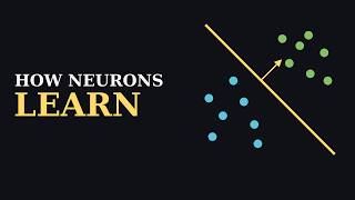
Linear separability splits the input space with one boundary. Points with positive response lie on one side. Points with negative response lie on the other. The boundary is also called the decision line.

The net input defines the sides:

z = \sum_{i=1}^{n} w_i x_i + w_0

$z \gt 0$ means a positive response. $z \lt 0$ means a negative response. The boundary is $z = 0$ .

\sum_{i=1}^{n} w_i x_i + w_0 = 0 \qquad\Longleftrightarrow\qquad \sum_{i=1}^{n} w_i x_i - t = 0 \qquad\Longleftrightarrow\qquad \sum_{i=1}^{n} w_i x_i = t

All three forms state the same boundary. The first uses the bias. The others use the threshold $t = -w_0$ .

Line, plane or hyperplane Search on YouTube

The input count sets the shape. Two inputs give a line. Three inputs give a plane. More inputs give a hyperplane.

w_1 x_1 + w_2 x_2 + w_0 = 0 \qquad\Longleftrightarrow\qquad y = mx + c \;\; \text{means} \;\; mx - y + c = 0

The left form is the two-input boundary. The right form recalls the school line $y = mx + c$ .

OR with a perceptron Search on YouTube

OR outputs $0$ only for $(0,0)$ . It outputs $1$ for $(1,0)$ , $(0,1)$ and $(1,1)$ . Write $x_0 = 1$ for the bias term. Then each row gives one inequality:

\begin{aligned} w_0 + w_1\cdot 0 + w_2\cdot 0 &\lt 0\\ w_0 + w_1\cdot 1 + w_2\cdot 0 &\ge 0\\ w_0 + w_1\cdot 0 + w_2\cdot 1 &\ge 0\\ w_0 + w_1\cdot 1 + w_2\cdot 1 &\ge 0 \end{aligned} \qquad\Longleftrightarrow\qquad \begin{aligned} w_0 &\lt 0\\ w_0 + w_1 &\ge 0\\ w_0 + w_2 &\ge 0\\ w_0 + w_1 + w_2 &\ge 0 \end{aligned}

$w_0$ is the bias. $w_1, w_2$ are the input weights. Any triple that satisfies all four rows implements OR.

OR is separable. The line through (1,0) and (0,1) leaves (0,0) alone.

Worked example: solve the OR inequalities. Pick $w_0 = -1$ , $w_1 = 1$ , $w_2 = 1$ .

\begin{aligned} (0,0):\quad -1 &\lt 0 \;\Rightarrow\; \mathbf{0}\\ (1,0):\quad -1 + 1 = 0 &\ge 0 \;\Rightarrow\; \mathbf{1}\\ (0,1):\quad -1 + 1 = 0 &\ge 0 \;\Rightarrow\; \mathbf{1}\\ (1,1):\quad -1 + 1 + 1 = 1 &\ge 0 \;\Rightarrow\; \mathbf{1} \end{aligned}

Read the boundary. The line is $x_1 + x_2 - 1 = 0$ . It cuts the axes at $(1,0)$ and $(0,1)$ . The triple $[-1, 2, 2]$ from the slides passes the same four tests.

Random weights and the error surface Search on YouTube

Fix the bias and vary $w_1, w_2$ . Each trial draws one decision line. The slides try several lines. One line makes $3$ errors. A better line makes $1$ error. The error surface bottoms out when both $w_1$ and $w_2$ exceed $1$ . Random search wastes trials there. A principled rule finds the weights directly.

Push a fence until each animal stands on the right side. Each mistake tells you which way to push. PLA turns each mistake into one push.

Perceptron learning algorithm Search on YouTube

The Perceptron Learning Algorithm (PLA) trains one perceptron for binary classification. $P$ is the positive class. $N$ is the negative class. $w$ is the weight vector (bias $w_0$ included). $x$ is the input vector (with $x_0 = 1$ ). PLA seeks the decision line that separates $P$ from $N$ . It stops when every input is classified correctly.

Predict $1$ when $z \ge 0$ . Predict $0$ when $z \lt 0$ . Update only on mistakes:

w \leftarrow w + x \quad \text{(true $1$, predicted $0$)} \qquad\qquad w \leftarrow w - x \quad \text{(true $0$, predicted $1$)}

Add the input when the perceptron misses a positive point. Subtract the input on a false alarm. Leave $w$ unchanged on correct predictions.

Memorise the directions: miss means add, false alarm means subtract. The bias $w_0$ updates too because $x_0 = 1$ rides along.

PLA for OR, step by step Search on YouTube

Start from $w = [-1, 0, 0]$ . Cycle the OR rows in order $(1,0)$ , $(0,1)$ , $(1,1)$ , $(0,0)$ . The slides show the first four computations. The trace below continues to convergence at $w = [-1, 1, 1]$ .

Steps 1 to 4: first pass. Current weights are $w = [-1, 0, 0]$ .

\begin{aligned} (1,0):\quad z &= -1\cdot 1 + 0\cdot 1 + 0\cdot 0 = -1 \lt 0 \;\Rightarrow\; \text{predict } \mathbf{0},\ \text{true } 1,\ \text{update}\\ w &= [-1+1,\ 0+1,\ 0+0] = \mathbf{[0, 1, 0]}\\ (0,1):\quad z &= 0\cdot 1 + 1\cdot 0 + 0\cdot 1 = 0 \ge 0 \;\Rightarrow\; \text{predict } \mathbf{1},\ \text{true } 1,\ \text{no update}\\ (1,1):\quad z &= 0\cdot 1 + 1\cdot 1 + 0\cdot 1 = 1 \ge 0 \;\Rightarrow\; \text{predict } \mathbf{1},\ \text{true } 1,\ \text{no update}\\ (0,0):\quad z &= 0\cdot 1 + 1\cdot 0 + 0\cdot 0 = 0 \ge 0 \;\Rightarrow\; \text{predict } \mathbf{1},\ \text{true } 0,\ \text{update}\\ w &= [0-1,\ 1-0,\ 0-0] = \mathbf{[-1, 1, 0]} \end{aligned}

Steps 5 to 8: second pass. Current weights are $w = [-1, 1, 0]$ .

\begin{aligned} (1,0):\quad z &= -1 + 1 + 0 = 0 \ge 0 \;\Rightarrow\; \text{predict } \mathbf{1},\ \text{true } 1,\ \text{no update}\\ (0,1):\quad z &= -1 + 0 + 0 = -1 \lt 0 \;\Rightarrow\; \text{predict } \mathbf{0},\ \text{true } 1,\ \text{update}\\ w &= [-1+1,\ 1+0,\ 0+1] = \mathbf{[0, 1, 1]}\\ (1,1):\quad z &= 0 + 1 + 1 = 2 \ge 0 \;\Rightarrow\; \text{predict } \mathbf{1},\ \text{true } 1,\ \text{no update}\\ (0,0):\quad z &= 0 \ge 0 \;\Rightarrow\; \text{predict } \mathbf{1},\ \text{true } 0,\ \text{update}\\ w &= [0-1,\ 1-0,\ 1-0] = \mathbf{[-1, 1, 1]} \end{aligned}

Step 9: verify convergence. Test all rows with $w = [-1, 1, 1]$ .

\begin{aligned} (1,0):\quad -1 + 1 &= 0 \ge 0 \;\Rightarrow\; \mathbf{1}\\ (0,1):\quad -1 + 1 &= 0 \ge 0 \;\Rightarrow\; \mathbf{1}\\ (1,1):\quad -1 + 1 + 1 &= 1 \ge 0 \;\Rightarrow\; \mathbf{1}\\ (0,0):\quad -1 &\lt 0 \;\Rightarrow\; \mathbf{0} \end{aligned}

All four rows match OR. PLA stops. The slide target $[-1, 2, 2]$ is another valid separator.

Convergence theorem Search on YouTube

The theorem answers one question: does PLA stop after finite steps? It stops when the two classes are linearly separable. It needs finite point sets. It tests the vectors cyclically, one after another.

Two sets $P$ and $N$ in $n$ -dimensional space are absolutely linearly separable when weights $w_0, w_1, \dots, w_n$ exist with:

\sum_{i=1}^{n} w_i x_i \gt -w_0 \quad \text{for every point in } P \qquad\qquad \sum_{i=1}^{n} w_i x_i \lt -w_0 \quad \text{for every point in } N

$P$ sits fully on the positive side. $N$ sits fully on the negative side. The same $w_0$ serves both lines.

Proposition: when $P$ and $N$ are finite and linearly separable, PLA updates the weight vector finitely many times. After finite steps $t$ , the vector $w_t$ separates the two sets.

Run PLA only on separable data. On overlapping classes it never settles. It cycles through mistakes without end.

Spam filter and XOR limit Search on YouTube

Real tasks often reduce to linear choices. The spam scenario uses two binary features. Feature $x_1 = 1$ when "free" appears. Feature $x_2 = 1$ when "win" appears. The slides label $(0,0)$ as safe. They label $(0,1)$ , $(1,0)$ and $(1,1)$ as spam. That table is OR. One perceptron implements it.

XOR breaks the perceptron. XOR outputs $1$ for $(0,1)$ and $(1,0)$ . It outputs $0$ for $(0,0)$ and $(1,1)$ . Opposite corners share labels. No single straight line isolates the two $1$ s.

XOR is not separable. The OR line leaves (1,1) on the wrong side.

Worked example: prove XOR needs more than one line. Assume a separator exists with $w_0 \lt 0$ for $(0,0)$ .

\begin{aligned} (0,0):\quad w_0 &\lt 0\\ (1,0):\quad w_0 + w_1 &\ge 0\\ (0,1):\quad w_0 + w_2 &\ge 0\\ (1,1):\quad w_0 + w_1 + w_2 &\lt 0 \end{aligned}

Derive the clash. Add the two middle rows.

\begin{aligned} 2w_0 + w_1 + w_2 &\ge 0\\ w_0 &= (2w_0 + w_1 + w_2) - (w_0 + w_1 + w_2) \gt 0 - 0 = 0 \end{aligned}

So $w_0 \gt 0$ . This clashes with $w_0 \lt 0$ . No triple satisfies all rows. XOR is nonlinear for one perceptron. Higher networks (with hidden layers) handle it.

Try PLA on OR and XOR below. Move the weights or press Play PLA and watch the line react.

Line is w1x1+w2x2+w0=0. Blue dots output 1. Hollow dots output 0.

Bias w0: -1Weight w1: 1Weight w2: 1

z = 1x1 + 1x2 + -1. Predict 1 when z ≥ 0.

Weights solve OR. Press Reset, then Play PLA. 4 of 4 rows pass. Mistakes: 0.

ANN layers Search on YouTube

The network stacks neurons in layers. The arrangement plus the connection pattern is the network architecture.

Neuron: a cell that sums weighted inputs, adds a bias and holds activity $a$ .
Input layer: the first layer. It receives the raw input vector. With $m$ dimensions, it holds $m$ neurons. Each neuron is a placeholder for one dimension (no computation).
First dense layer in Keras: each neuron takes the full input vector. Its size need not equal the input size. The slides contrast this practical layout with the placeholder view.
Hidden layer: any layer between input and output. It extracts patterns from its inputs. Each layer may hold a different neuron count.
Output layer: the last layer. It emits one or more values from the previous layer.

A first input vector $I_1 = \{x_{11}, x_{12}, x_{13}\}$ feeds three input neurons in the slide sketch. Each dense neuron would instead see the whole triple.

Three aspects of a model Search on YouTube

Slide lists three model aspects: synaptic interconnections, training rules for weight updates and activation functions. Later lectures vary each aspect.

Feedforward and feedback networks Search on YouTube

Interconnections fall in two groups: feedforward and feedback.

Feedforward	Feedback
Data flow one way (input to hidden to output)	Outputs return as inputs (same or earlier layer)
No cycles or loops	Loops carry past information forward
Sequential Dense models	Recurrent and dynamic networks
Fixed-size classification and regression	Sequences: time series, language, speech

Feedforward types: single-node network (linear perceptron), single-layer network and multilayer network. Feedback types: single node with self-feedback, single-layer recurrent network and multilayer recurrent network. Lateral feedback returns output within the same layer. It models competition or cooperation (stronger neurons suppress weaker ones through lateral inhibition). Self-feedback returns one output to its own neuron. Cross-neuron feedback sends outputs to other neurons in the same or earlier layers. Recurrent neural networks (RNNs) process sequences with such loops. Variants named in the slides: LSTM, GRU and bidirectional RNNs. A single-layer perceptron has no hidden layer (input to output). Its output layer may hold several perceptrons. A multilayer perceptron (MLP) adds hidden layers. It handles linear and nonlinear functions.

F-F-F, F-R-M: loops or no loops

Feedforward: single-node, single-layer, multilayer (no loops) · Feedback: self, recurrent single-layer, multilayer (loops back).

Quick self-test Search on YouTube

1. Map each artificial part (input, weight, sum, activation, output) to its biological part.

Inputs map to dendrites. Weights map to synaptic strength. Sum maps to the cell body. Activation maps to firing. Output maps to the axon.

2. Differentiate the MP neuron from the Rosenblatt perceptron in three points.

MP uses Boolean inputs and fixed weights with no learning. The perceptron accepts real inputs and learns weights and bias. MP sets the threshold by hand, while the perceptron shifts it through $w_0$ .

3. Weights are

1, 1

with threshold

2

. Compute the outputs for

(0,1)

and

(1,1)

. Which gate is it?

$(0,1)$ sums to $1 \lt 2$ , so output is $0$ . $(1,1)$ sums to $2 \ge 2$ , so output is $1$ . The full table is AND.

4. Solve for OR: which inequality does

(0,0)

give, and does

w = [-1, 1, 1]

satisfy all rows?

$(0,0)$ gives $w_0 \lt 0$ . The triple gives $-1$ , $0$ , $0$ , $1$ across the four rows. All four tests pass, so it implements OR.

5. Starting from

w = [-1, 0, 0]

, what is

z

for OR input

(1,0)

and what is the update?

$z = -1 \lt 0$ predicts $0$ against true $1$ . Add the input: $w$ becomes $[0, 1, 0]$ .

6. With

w = [0, 1, 0]

, what does PLA do on OR input

(0,0)

, and why?

$z = 0 \ge 0$ predicts $1$ against true $0$ . Subtract the input $[1, 0, 0]$ : $w$ becomes $[-1, 1, 0]$ . Subtraction fixes false alarms.

7. Compute

\sigma(-0.9)

and

\sigma(0.7)

to three decimals. What trend do they show?

$\sigma(-0.9) = 0.289$ and $\sigma(0.7) = 0.668$ . Activity rises with $z$ . The sigmoid grades the response instead of switching hard.

8. Three step neurons give how many patterns, and three 10-level sigmoid neurons give how many?

Step gives $2^3 = 8$ patterns. Graded gives $10^3 = 1000$ patterns. More levels expand the solution space.

9. Why does PLA converge on OR but never settle on overlapping classes?

OR is linearly separable, so a separator exists and PLA makes finite updates. Overlapping classes admit no separator, so mistakes never end and updates cycle forever.

10. Prove with four inequalities that no single perceptron implements XOR.

XOR needs $w_0 \lt 0$ , $w_0 + w_1 \ge 0$ , $w_0 + w_2 \ge 0$ , $w_0 + w_1 + w_2 \lt 0$ . The middle rows force $w_0 \gt 0$ . The clash proves the need for hidden layers.

The artificial neuron copies biology: inputs (dendrites), weights (synapses), sum (cell body), activation (firing), output (axon).
The MP neuron (McCulloch and Pitts, 1943) uses Boolean inputs and a fixed threshold. It learns nothing.
AND with weights $1, 1$ needs threshold $2$ . Only $(1,1)$ reaches it.
The perceptron (Rosenblatt, 1958) learns weights and bias. It handles only linear boundaries.
Step gives hard $0$ or $1$ . Sigmoid $\sigma(z) = 1/(1+e^{-z})$ grades activity (for example $\sigma(0.7) = 0.668$ ).
Bias form: $z = \sum w_i x_i + w_0$ with $w_0 = -t$ . Fire when $z \ge 0$ .
The boundary is $\sum w_i x_i + w_0 = 0$ . Two inputs give a line, three give a plane, more give a hyperplane.
OR needs $w_0 \lt 0$ , $w_0+w_1 \ge 0$ , $w_0+w_2 \ge 0$ , $w_0+w_1+w_2 \ge 0$ . Both $[-1,1,1]$ and $[-1,2,2]$ pass.
PLA adds the input on a miss and subtracts it on a false alarm. It stops when all rows pass.
PLA converges in finite steps only for finite linearly separable sets. XOR is the canonical failure ( $\mathbf{w_0 \lt 0}$ clashes with $\mathbf{w_0 \gt 0}$ ).

Perceptron & linear separability

Biological neuron to artificial neuronSearch on YouTubeBookmarkSaved

Computational unitsSearch on YouTubeBookmarkSaved

McCulloch-Pitts neuronSearch on YouTubeBookmarkSaved

Threshold logicSearch on YouTubeBookmarkSaved

MP neuron featuresSearch on YouTubeBookmarkSaved

Supervised learningSearch on YouTubeBookmarkSaved

Classification and regressionSearch on YouTubeBookmarkSaved

Linear perceptronSearch on YouTubeBookmarkSaved

Step and sigmoid activationSearch on YouTubeBookmarkSaved

Step functionSearch on YouTubeBookmarkSaved

SigmoidSearch on YouTubeBookmarkSaved

Patterns in solution spaceSearch on YouTubeBookmarkSaved

From threshold to biasSearch on YouTubeBookmarkSaved

Training: loss and weight updatesSearch on YouTubeBookmarkSaved

Linear separabilitySearch on YouTubeBookmarkSaved

Line, plane or hyperplaneSearch on YouTubeBookmarkSaved

OR with a perceptronSearch on YouTubeBookmarkSaved

Random weights and the error surfaceSearch on YouTubeBookmarkSaved

Perceptron learning algorithmSearch on YouTubeBookmarkSaved

PLA for OR, step by stepSearch on YouTubeBookmarkSaved

Convergence theoremSearch on YouTubeBookmarkSaved

Spam filter and XOR limitSearch on YouTubeBookmarkSaved

ANN layersSearch on YouTubeBookmarkSaved

Three aspects of a modelSearch on YouTubeBookmarkSaved

Feedforward and feedback networksSearch on YouTubeBookmarkSaved

Quick self-testSearch on YouTubeBookmarkSaved

On this page