RNN & backprop through time

This lecture processes ordered data with a recurrent network. It shares one set of weights across time steps and trains them with backprop through time. After this page you can run a two-step RNN forward pass by hand and trace one BPTT gradient.

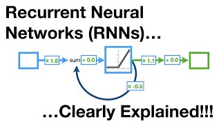RNNs Clearly ExplainedStatQuest · Sequence recurrence unfolding intuition

RNNs Image Captioning LSTMAndrej Karpathy · RNN LSTM vanishing gradients

Sequence learning Search on YouTube

Feedforward networks and CNNs take fixed-size inputs. They treat every input as independent of the others. Sequence tasks break both rules. Length varies from sample to sample. Order changes the meaning.

The slides show auto word prediction. Feed d into the network and it predicts e. Feed that e back in and it predicts the next letter. Each prediction depends on the letters seen before.

Two more slide tasks work the same way. POS tagging assigns one tag to each word in order. Polarity scoring reads a whole review and outputs one label.

A sentence is a queue, not a bag of coins. Shuffle the words and the total stays the same, but the meaning breaks.

Sequence learning covers problems with ordered, variable-length input. Temporal dependence means the current input needs the past inputs for its meaning. Speech, text, sensor traces and video are natural examples.

Challenges in sequence learning Search on YouTube

Three demands separate sequence learning from standard learning:

Variable-length inputs. Sentences and traces have different lengths. The model must accept any length.
Temporal dependencies. The meaning of the current input depends on previous elements. not flips the good that follows it.
Same function at each time step. The model must reuse one parameter set for every time step $t$ . Sharing cuts the parameter count and helps the model generalize across time.

Failed alternatives Search on YouTube

Two naive designs fail before the RNN appears.

First, reuse one fixed network per element with no memory. It accepts any length. It keeps no dependency on previous inputs. Each step sees only the current element.

Second, train separate weights for each position. Position 1 gets one matrix, position 2 another, and so on. The parameter count grows with length. Computation grows with it. Long sentences become untrainable.

Approach	Any length	Keeps history	Parameter cost
Fixed net, no memory	yes	no	small
One net per position	no	yes	grows with length
RNN with shared weights	yes	yes	fixed

S0, S1 and S2 solution Search on YouTube

The slides build the fix from states. Keep a state $S$ that summarizes the past. Update it at each step. Read the output $O$ from it.

The chain runs $S_0 \to S_1 \to S_2$ . Each new state combines the current input with the previous state. The output at each step reads the current state. This is the recurrent solution. The next section names the pieces.

Recurrent neural network Search on YouTube

An RNN processes a sequence one element at a time. It keeps a hidden state that carries past information forward. The hidden state (the slides also call it state $S_t$ ) updates at every step with the same weights.

Unrolled RNN over three steps. U feeds inputs in, W carries the state forward, V reads outputs out.

h_t = \sigma(U x_t + W h_{t-1} + b)

$h_t$ is the hidden state at step $t$ . $x_t$ is the input at step $t$ . $U$ maps inputs to the hidden state. $W$ maps the previous hidden state to the current one. $b$ is the bias. $\sigma$ is the hidden activation function.

\hat{y}_t = O_t(V h_t + c)

$\hat{y}_t$ is the predicted value at step $t$ ( $y_t$ is the label). $V$ maps the hidden state to the output. $c$ is the output bias. $O_t$ is the output activation function: softmax, sigmoid or linear.

The same $U$ , $W$ , $V$ , $b$ and $c$ serve every step. Sharing is what keeps the model small. The hidden state is the only thing that changes with time.

Training a recurrent network Search on YouTube

Training follows three steps. They mirror feedforward training, with time added.

Run the forward pass. Feed the sequence step by step. Update the hidden state and emit outputs.
Compute the loss. Compare each prediction with its label. Add the per-step losses into one total.
Run backprop through time. Send gradients back across steps. Add them and update the weights.

Outputs appear at each step or only at the final step. Tagging needs one output per step. Polarity needs only the last one.

L = \sum_{t=1}^{T} L_t

$L$ is the total loss over a sequence of length $T$ . $L_t$ is the loss at step $t$ . All learnable parameters sit in $\theta = \{V, W, U\}$ plus biases.

L_t = \tfrac{1}{2}(y_t - \hat{y}_t)^2 \qquad L_t = -\sum_i y_{t,i}\log \hat{y}_{t,i}

Use squared error for real-valued targets. Use cross entropy for class targets. $O_t$ pairs with the loss: linear with squared error, sigmoid with binary labels, softmax with cross entropy.

Worked example. Scalar toy RNN, two steps. Weights $U = 0.6$ , $W = 0.8$ , $V = 1.0$ , biases $0$ . Inputs $x_1 = 1$ , $x_2 = 0.5$ . Start state $h_0 = 0$ . Hidden and output activations are sigmoid.

Step 1. $a_1 = 0.6 \cdot 1 + 0.8 \cdot 0 = 0.6$ .

\begin{aligned} h_1 &= \sigma(0.6) = 1/(1+e^{-0.6}) = 1/1.5488 = \mathbf{0.6457} \end{aligned}

Step 2. $a_2 = 0.6 \cdot 0.5 + 0.8 \cdot 0.6457 = 0.3 + 0.5166 = 0.8166$ .

\begin{aligned} h_2 &= \sigma(0.8166) = 1/(1+e^{-0.8166}) = 1/1.4420 = \mathbf{0.6935}\\ \hat{y}_2 &= \sigma(1.0 \cdot 0.6935) = 1/(1+e^{-0.6935}) = 1/1.4998 = \mathbf{0.6668} \end{aligned}

Check. $e^{-0.6} = 0.5488$ , $e^{-0.8166} = 0.4420$ , $e^{-0.6935} = 0.4998$ . Recompute each quotient and the digits match.

Backprop through time Search on YouTube

BPTT is backprop unrolled over time. It computes one gradient per step and adds them. Shared weights collect their updates from all steps.

Time order controls the chain rule. $h_t$ depends on $W$ twice over. The direct path is the $W h_{t-1}$ term inside $h_t$ . The indirect path runs through $h_{t-1}$ , which itself used $W$ . The same split holds for $U$ .

\frac{\partial L}{\partial W} = \sum_{t=1}^{T} \frac{\partial L_t}{\partial W} \qquad \frac{\partial L}{\partial U} = \sum_{t=1}^{T} \frac{\partial L_t}{\partial U}

Each step contributes its own gradient. Shared weights sum them. $h_0$ is a constant, so its derivative is $0$ .

\frac{\partial L_t}{\partial W} = \frac{\partial L_t}{\partial \hat{y}_t}\frac{\partial \hat{y}_t}{\partial h_t} \sum_{r=1}^{r \le t}\left(\prod_{k=r+1}^{t}\frac{\partial h_k}{\partial h_{k-1}}\right)\left(\frac{\partial h_r}{\partial W}\right)_{\text{explicit}}

The explicit part is the direct use of $W$ at step $r$ . The implicit part is the product chain back through $h_{r+1} \dots h_t$ . The $U$ gradient reuses the same chain with $(\partial h_r / \partial U)$ in place of $(\partial h_r / \partial W)$ .

The $r = t$ term is the explicit component. Terms with $r \lt t$ are implicit components. They trace back to $h_1$ . The $r = 0$ term drops out because $h_0$ is constant.

Trace one $L_t$ at a time in exams. Write the output path first. Then expand one explicit term plus one implicit chain. Examiners award marks for the split.

Worked example. BPTT trace for $L_2$ with the toy numbers above. Loss $L_2 = \tfrac{1}{2}(y_2 - \hat{y}_2)^2$ with label $y_2 = 1$ and $\hat{y}_2 = 0.6668$ .

Output path. Error signal times sigmoid slope.

\begin{aligned} \partial L_2/\partial \hat{y}_2 &= 0.6668 - 1 = -0.3332\\ \partial \hat{y}_2/\partial h_2 &= 0.6668 \cdot 0.3332 = 0.2222\\ \partial L_2/\partial h_2 &= -0.3332 \cdot 0.2222 = \mathbf{-0.0740} \end{aligned}

Hidden path. Sigmoid slopes: $\sigma^\prime(a_2) = 0.6935 \cdot 0.3065 = 0.2126$ .

\begin{aligned} (\partial h_2/\partial W)_{\text{explicit}} &= 0.2126 \cdot h_1 = 0.2126 \cdot 0.6457 = \mathbf{0.1373}\\ \partial h_2/\partial h_1 &= 0.2126 \cdot 0.8 = \mathbf{0.1701}\\ (\partial h_1/\partial W)_{\text{explicit}} &= \sigma^\prime(a_1) \cdot h_0 = 0 \;\; (h_0 = 0) \end{aligned}

Combine. Implicit term dies on $h_0 = 0$ . Only the explicit term at $r = 2$ stays.

\begin{aligned} \partial L_2/\partial W &= -0.0740 \cdot (0.1373 + 0.1701 \cdot 0) = \mathbf{-0.0102} \end{aligned}

Check. $0.6935 \cdot 0.3065 = 0.2126$ . Then $0.2126 \cdot 0.6457 = 0.1373$ . Then $0.0740 \cdot 0.1373 = 0.0102$ . Signs stay negative, so gradient descent raises $W$ .

The lab replays the two-step scalar RNN from the worked example. It then traces the BPTT chain and the clip plus truncate fixes.

Unrolled toy RNN. U, W and V stay shared across steps.

a2 = 0.3 + 0.5166 = 0.8166. h2 = 0.6935. y-hat = 0.6668.

Step factor |W| x slope: 0.25

0.25^5 = 0.0010 (0.25^5 is about 0.001). Signal vanishes.

Clip ceiling tau: 5

Norm is 12. Scale is 0.4167. Clipped norm is 5.0.

Truncate history k: 2 of 7 steps

k = 2 keeps steps 6 to 7. Older links stay unlearned.

Vanishing and exploding gradients Search on YouTube

The implicit chain multiplies many derivatives. Each factor is a Jacobian $\partial h_k / \partial h_{k-1} = \sigma^\prime(a_k)\,W$ . Long products misbehave in two ways.

Vanishing means gradients shrink step by step. Early steps barely update. Learning stalls. Sigmoid slopes peak at $0.25$ . Tanh slopes peak at $1.0$ . Products of such factors decay fast.

Exploding means gradients grow step by step. Weights blow up. Training turns unstable. Factors above $1$ compound the same way in reverse.

\frac{\partial h_t}{\partial h_{t-k}} = \prod_{j=0}^{k-1} \sigma^\prime(a_{t-j})\,W

Saturation adds to the damage. Large $|w|$ makes the sigmoid switch too fast. Large $|b|$ shifts it left or right into a flat end. Flat ends have near-zero slope, so gradients vanish there too.

Vanishing	Exploding
Gradients shrink toward 0	Gradients grow out of control
Early steps stop learning	Weights blow up, loss jumps
Caused by slopes below 1, saturation	Caused by factors above 1
Fix: truncate history, gate memory	Fix: clip gradients

Fixes: clipping and truncated BPTT Search on YouTube

The slides name three fixes. The first two belong here. The third is a later lecture.

Gradient clipping caps exploding steps. Pick a ceiling $\tau$ such as $1$ or $5$ . Rescale any gradient above it. Direction stays the same. Size stops at $\tau$ .

Truncated BPTT caps the history length. Backpropagate only $k$ steps. A 100-word sequence might train on the last 20 steps. Long-range links beyond $k$ go unlearned. Cost per update stays flat.

LSTM adds a memory cell for long-range links. It is the topic of the next lecture.

g \leftarrow g \cdot \min\left(1,\, \tau / \Vert g \Vert\right)

$g$ is the gradient vector. $\Vert g \Vert$ is its norm. $\tau$ is the ceiling. Gradients below $\tau$ pass through unchanged.

C-T-L: Clip, Truncate, LSTM

Clip caps gradient size · Truncate caps history length · LSTM (next lecture) carries long memory.

Truncate with care on exams. A small $k$ speeds training but erases links longer than $k$ . Name the trade-off when you recommend it.

Bag of words for text classification Search on YouTube

The classic pipeline ignores order. Tokenize the text. Build a vocabulary with one index per word. Count words per document into a design matrix. Feed the matrix to a plain classifier.

Each row is one document. Each column is one word. Cell values are counts or term frequencies. Labels sit in a vector $Y$ .

Worked example. Three reviews. Vocabulary: movie (0), is (1), good (2), not (3). Labels: $1$ for positive, $0$ for negative.

Doc	Text	movie	is	good	not	$Y$
d1	movie is good	1	1	1	0	1
d2	movie is not good	1	1	1	1	0
d3	not good	0	0	1	1	0

Read it. The design matrix is $3 \times 4$ . $Y$ is $3 \times 1$ . Row d3 equals the counts of good not. Order is lost: not good and good not share one row.

The slide pair proves the loss. The movie my friend has not seen is good is positive. The movie my friend has seen is not good is negative. Both use the same word multiset. Their count rows match. A BoW classifier cannot split them.

RNN text classification Search on YouTube

The RNN pipeline keeps order. Map words to integer ids. Pad short sentences to one length. Replace ids with vectors. Feed the vectors step by step.

Integers alone mislead. Id $7$ is not larger than id $2$ . One-hot vectors remove the fake order. Each word becomes a sparse $1 \times V$ row with one $1$ .

Dense embeddings replace the sparse rows. The embedding matrix $E$ has size $V \times D$ . $V$ is the vocabulary size. $D$ is the embedding size (feature count per word). Rows come from Word2Vec, GloVe, FastText or training from scratch.

The lookup trick skips the sparse multiply. $(1 \times V)$ times $(V \times D)$ gives $(1 \times D)$ . That product copies one row of $E$ . So gather rows by index instead of multiplying.

e = x_{\text{one-hot}}\,E \qquad (1 \times V)\,(V \times D) = (1 \times D)

$x_{\text{one-hot}}$ is one $1 \times V$ word vector. $E$ is the $V \times D$ embedding matrix. $e$ is the $1 \times D$ dense word vector. Lookup copies row $i$ of $E$ when the $1$ sits at index $i$ .

Worked example. Vocabulary size $V = 11$ (ids $0$ to $9$ , pad id $10$ ). Embedding size $D = 4$ . Sentence ids $[7, 5, 2, 4]$ padded to length $7$ with $[10, 10, 10]$ .

Lookup. Copy rows of $E$ in token order. Pad rows are zeros.

\begin{aligned} \text{row } 7 &= [1, 0, 2, 0]\\ \text{row } 5 &= [0, 1, 1, 0]\\ \text{row } 2 &= [2, 2, 0, 1]\\ \text{row } 4 &= [0, 0, 1, 2]\\ \text{row } 10 &= [0, 0, 0, 0] \end{aligned}

Stack. Four word rows plus three pad rows give a $7 \times 4$ input matrix.

1	0	2	0
0	1	1	0
2	2	0	1
0	0	1	2
0	0	0	0
0	0	0	0
0	0	0	0

Check. Full one-hot math would multiply $(7 \times 11)$ by $(11 \times 4)$ to get $(7 \times 4)$ . Lookup copies the same $7$ rows. Dims and values agree.

Out-of-vocabulary words need a plan. Map unseen words to one unknown vector. Or build their vectors from sub-word pieces. A fresh Word2Vec trained only on new words may land in a different space, so avoid that shortcut.

Character prediction with vocab E S T Search on YouTube

Character RNNs use a tiny vocabulary. Here it is $\{E, S, T\}$ with size $3$ . Inputs are one-hot: $E = [1,0,0]$ , $S = [0,1,0]$ , $T = [0,0,1]$ . Possible words include SET, SEE, SETS, SEES and TEST. A full capital-letter vocabulary would need size $26$ .

The model reads one character per step. It predicts the next character. Softmax over $3$ logits gives the probabilities.

P(y = i \vert z) = e^{z_i}/\sum_j e^{z_j} \qquad L_t = -\log P(y = \text{label} \vert z)

$z$ holds the $3$ logits. $P$ is the predicted probability per character. $L_t$ is the cross entropy loss at step $t$ for the true next character.

Worked example. Input so far: S E E. True next character: S (spells SEES). Logits for $[E, S, T]$ are $z = [1.2,\, 2.0,\, 0.5]$ .

Softmax. Exponentiate and normalize.

\begin{aligned} e^{1.2} &= 3.3201 \qquad e^{2.0} = 7.3891 \qquad e^{0.5} = 1.6487\\ \text{sum} &= 3.3201 + 7.3891 + 1.6487 = 12.3579\\ P(E) &= 3.3201/12.3579 = \mathbf{0.2687}\\ P(S) &= 7.3891/12.3579 = \mathbf{0.5979}\\ P(T) &= 1.6487/12.3579 = \mathbf{0.1334} \end{aligned}

Decide and score. Max probability is $S$ , so the model emits S. Loss is $-\log(0.5979) = \mathbf{0.5144}$ . Probabilities sum to $1.0000$ .

RNN variants Search on YouTube

One recurrence serves many layouts. The layout follows the task.

Sentiment and document classification is many-to-one. The RNN reads one word vector $x_t$ per step. It updates $h_t$ from $x_t$ and $h_{t-1}$ . After the last word, one vector $y$ passes through softmax into positive, negative or neutral.

Image captioning is one-to-many. A CNN encoder (such as ResNet) turns the image into a vector $v$ . $v$ seeds the initial hidden state $h_0$ . The RNN then emits words. Step 1 takes a start token and outputs $y_1$ . Step 2 takes $y_1$ and outputs $y_2$ . Decoding stops at an end token or a max length.

POS tagging is many-to-many and aligned. Each word maps to its tag at the same step. Input count equals output count. No delay.

Translation and question answering is many-to-many with delay. The RNN reads the full input first. Outputs start only after encoding ends. Alignment across languages is not one-to-one.

Variant	Layout	Outputs start
Sentiment scoring	many-to-one	after last word
Image captioning	one-to-many	after image vector seeds $h_0$
POS tagging	many-to-many, aligned	at same step
Translation	many-to-many, delayed	after full input

Quick self-test Search on YouTube

1. Why do feedforward nets fail on The movie my friend has not seen is good vs ... has seen is not good?

Both sentences share one word multiset, so fixed-size count inputs match. Order carries the flip from not. Sequence models read order, so they split the pair.

2. Scalar RNN with

U = 0.5

W = 0.5

b = 0

h_0 = 0

. Input

x_1 = 2

. Find

h_1

with sigmoid.

$a_1 = 0.5 \cdot 2 + 0.5 \cdot 0 = 1.0$ . $h_1 = \sigma(1.0) = 1/(1 + e^{-1}) = 1/1.3679 = 0.7311$ .

3. Per-step losses are

L_1 = 0.2

L_2 = 0.5

L_3 = 0.1

. What total does BPTT differentiate?

$L = 0.2 + 0.5 + 0.1 = 0.8$ . BPTT sums per-step gradients of this total.

4. Differentiate the explicit and implicit parts of

\partial L_t / \partial W

Explicit is the direct $W$ use at step $r$ . Implicit is the chain back through $h_{r+1} \dots h_t$ . The $r = t$ term is purely explicit.

5. Each step multiplies the gradient by

0.25

. How much survives after

5

steps back?

$0.25^5 = 0.00098 \approx 0.001$ . Only about a thousandth survives. That is vanishing in numbers.

6. Gradient norm is

12

and the ceiling is

\tau = 5

. What scale factor applies?

Factor $= 5/12 = 0.4167$ . New norm is $5$ . Direction is unchanged.

7. Vocabulary order: movie, is, good, not. Write the BoW row for movie not good. What label breaks BoW here?

Row is $[1, 0, 1, 1]$ . good not gives the same row with opposite sense. Counts cannot split them.

8. Vocab size

9

, embedding size

6

5

tokens in. What tensor feeds the RNN?

Each token gives $1 \times 6$ . Five tokens stack to $5 \times 6$ . Lookup skips the $(5 \times 9)(9 \times 6)$ multiply.

9. Logits

[E, S, T] = [0.5, 1.5, 0.0]

. Which character wins, with what probability?

Exponentials: $1.6487$ , $4.4817$ , $1.0$ . Sum $= 7.1304$ . $P = [0.2312, 0.6285, 0.1403]$ . $S$ wins at $0.6285$ .

10. POS tagging vs translation: which emits outputs with a delay, and why?

Translation waits for the full input first. Its outputs align with encoded meaning, not with input positions. POS tagging emits at the same step instead.

Sequence tasks have variable length and order-dependent meaning. Fixed independent inputs fail them.
Failed options are memory-free reuse (no history) and per-position weights (too many parameters).
The RNN updates $h_t = \sigma(Ux_t + Wh_{t-1} + b)$ and predicts $\hat{y}_t = O_t(Vh_t + c)$ with shared weights.
Training runs forward pass, total loss $L = \sum L_t$ , then BPTT sums per-step gradients.
BPTT splits each gradient into explicit (direct $W$ use) and implicit (chain through past states) parts.
Long chains vanish (factors below 1, saturation) or explode (factors above 1).
Fixes are gradient clipping ( $g \cdot \min(1, \tau/\Vert g\Vert)$ ), truncated BPTT (last $k$ steps) and LSTM memory (next lecture).
BoW counts words into a design matrix but loses order (not good equals good not).
RNN text input runs integers to padding to one-hot to embedding lookup $(1 \times V)(V \times D) = (1 \times D)$ .
Char prediction over $\{E,S,T\}$ uses softmax $e^{z_i}/\sum_j e^{z_j}$ ; the SEES example gives $P(S) = 0.5979$ and loss $0.5144$ .
Variants: sentiment (many-to-one), captioning (one-to-many from $h_0 = v$ ), POS (aligned), translation (delayed).

RNN & backprop through time

Sequence learningSearch on YouTubeBookmarkSaved

Challenges in sequence learningSearch on YouTubeBookmarkSaved

Failed alternativesSearch on YouTubeBookmarkSaved

S0, S1 and S2 solutionSearch on YouTubeBookmarkSaved

Recurrent neural networkSearch on YouTubeBookmarkSaved

Training a recurrent networkSearch on YouTubeBookmarkSaved

Backprop through timeSearch on YouTubeBookmarkSaved

Vanishing and exploding gradientsSearch on YouTubeBookmarkSaved

Fixes: clipping and truncated BPTTSearch on YouTubeBookmarkSaved

Bag of words for text classificationSearch on YouTubeBookmarkSaved

RNN text classificationSearch on YouTubeBookmarkSaved

Character prediction with vocab E S TSearch on YouTubeBookmarkSaved

RNN variantsSearch on YouTubeBookmarkSaved

Quick self-testSearch on YouTubeBookmarkSaved

On this page