Feedforward networks and gradient descent

This lecture builds a two-layer network of perceptrons that solves XOR. It then trains a sigmoid neuron with gradient descent. After this page you can compute a gradient-descent weight update by hand. You can also pick the loss that fits the task.

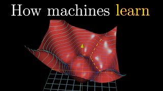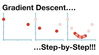How neural networks learn3Blue1Brown · GD intuition visual derivation

Gradient Descent Step-by-StepStatQuest · GD derivation step by step

Cross EntropyStatQuest · Classification loss cross-entropy

SGD Clearly ExplainedStatQuest · Stochastic GD mini-batch

The king's wine puzzle Search on YouTube

A king receives 1000 gift bottles of wine. Exactly one bottle is poisoned. Anyone who drinks it dies exactly 8 hours later. The feast starts in 9 hours, so only one round of testing is possible. The king has 10 prisoners for the tests. The task is to find the poisoned bottle with these 10 testers.

Each prisoner gives one yes-or-no answer: dead or alive. Ten answers form a 10-bit code. The Bottle labels are the code words.

Ten binary answers give $2^{10} = 1024$ patterns. That covers all 1000 bottles. Number the bottles from 0 to 999 in binary. Each bottle label has 10 bits. Prisoner $i$ sips from every bottle whose bit $i$ equals 1. After 8 hours the death pattern spells the poisoned bottle in binary.

Worked example. Bottle 637 is poisoned. Find which prisoners die.

Step 1. Write 637 in binary.

\begin{aligned} 637 &= 512 + 64 + 32 + 16 + 8 + 4 + 1\\ &= 2^9 + 2^6 + 2^5 + 2^4 + 2^3 + 2^2 + 2^0\\ \text{bits set} &= \{0, 2, 3, 4, 5, 6, 9\}\\ \text{label} &= \mathbf{1001111101} \end{aligned}

Step 2. Read the deaths. Prisoners 0, 2, 3, 4, 5, 6 and 9 die. Prisoners 1, 7 and 8 live. The pattern is 1001111101, which equals $512 + 64 + 32 + 16 + 8 + 4 + 1 = \mathbf{637}$ .

One yes-or-no unit carries one bit of information. A perceptron network works the same way. It combines many small yes-or-no units into one decision.

Networks of perceptrons Search on YouTube

A single perceptron cannot separate the XOR points. No single straight line does the job. A network of perceptrons can. It dedicates one hidden unit to each input pattern. Then the output unit fires for the wanted patterns.

Layers of the network Search on YouTube

The network has 3 layers. The input layer holds $x_1$ and $x_2$ . The hidden layer holds 4 perceptrons with outputs $h_1, h_2, h_3, h_4$ . The output layer holds one neuron with output $y$ . The input-to-hidden connections are the layer 1 weights. The hidden-to-output connections $w_1, w_2, w_3, w_4$ are the layer 2 weights.

Two inputs feed four hidden units. Each hidden unit watches one input pattern. One output unit reads the four hidden units.

One hidden unit per input pattern Search on YouTube

Each hidden perceptron fires for exactly one input pattern. No two units fire for the same input. Use bipolar inputs $\{-1, 1\}$ . The unit for pattern $(a, b)$ takes weights $(a, b)$ . It fires when the weighted sum exceeds 1. A matching pattern gives $1 + 1 = 2$ . A one-bit mismatch gives $1 - 1 = 0$ . A full mismatch gives $-2$ . Only the match passes the threshold.

h_k = 1 \text{ if } a_k x_1 + b_k x_2 \gt 1, \text{ else } 0

$(a_k, b_k)$ is the pattern of unit $k$ . At most one hidden unit fires at a time.

Unit	Pattern $(a, b)$	Weights	Fires for
$h_1$	$(-1, -1)$	$(-1, -1)$	$\{-1, -1\}$
$h_2$	$(-1, 1)$	$(-1, 1)$	$\{-1, 1\}$
$h_3$	$(1, -1)$	$(1, -1)$	$\{1, -1\}$
$h_4$	$(1, 1)$	$(1, 1)$	$\{1, 1\}$

XOR output weights Search on YouTube

The output neuron fires when $w_1 h_1 + w_2 h_2 + w_3 h_3 + w_4 h_4$ exceeds $w_0$ . The slides call $w_0$ the threshold. It equals the negative bias. XOR is true for patterns 2 and 3 only. So set the layer 2 weights to $(0, 1, 1, 0)$ with $w_0 = 0.5$ . The output is an OR of $h_2$ and $h_3$ .

y = 1 \text{ if } \sum_{i=1}^{4} w_i h_i \gt w_0, \text{ else } 0

$w_i$ are the layer 2 weights. $w_0$ is the threshold of the output neuron.

Worked example. Trace XOR with weights $(0, 1, 1, 0)$ and $w_0 = 0.5$ .

Step 1. Hidden units. Each input fires exactly one hidden unit.

$(x_1, x_2)$	$h_1$	$h_2$	$h_3$	$h_4$	Sum $0h_1 + h_2 + h_3 + 0h_4$	$y$
$(-1, -1)$	1	0	0	0	0	0
$(-1, 1)$	0	1	0	0	1	1
$(1, -1)$	0	0	1	0	1	1
$(1, 1)$	0	0	0	1	0	0

Step 2. Compare with 0.5. Sums of 1 exceed 0.5, so $y = 1$ . Sums of 0 do not, so $y = 0$ . The output column equals XOR.

For $n$ binary inputs there are $2^n$ patterns. Use $2^n$ hidden units (one per pattern) plus 1 output unit. The slides print "2n", but the example proves the exponent: 2 inputs need 4 units.

The slides note a smaller alternative construction for XOR. It uses fewer hidden units. The idea above is the general one: it works for any Boolean function.

Learnable parameters Search on YouTube

A fixed network solves logic by hand design. Learning finds the weights from data. Train one sigmoid neuron on two points: $(x_1, y_1) = (0.5, 0.2)$ and $(x_2, y_2) = (2.5, 0.9)$ . Find $w$ and $b$ with $f(0.5) \to 0.2$ and $f(2.5) \to 0.9$ . The learnable parameters are the weight $w$ and the bias $b$ .

The neuron output uses the sigmoid activation function:

f(z) = \sigma(z) = \frac{1}{1 + e^{-z}}, \qquad z = wx + b

$w$ is the weight and $b$ is the bias. The output lies between 0 and 1.

Fit quality uses the mean squared error loss:

L = \frac{1}{n}\sum_{i=1}^{n}(\hat{y}_i - y_i)^2, \qquad n = 2

$\hat{y}_i = f(x_i)$ is the predicted value. $y_i$ is the label. This loss is per-sample error averaged over samples.

Start with random values $w = 0.5$ and $b = 0$ .

Worked example. Compute the loss at $w = 0.5$ , $b = 0$ .

Step 1. First point $x_1 = 0.5$ . $z_1 = 0.5 \cdot 0.5 + 0 = 0.25$ .

\begin{aligned} f_1 &= 1/(1 + e^{-0.25}) = 1/1.7788 = 0.5622\\ \text{error}_1 &= 0.5622 - 0.2 = 0.3622\\ \text{error}_1^2 &= 0.3622^2 = \mathbf{0.1312} \end{aligned}

Step 2. Second point $x_2 = 2.5$ . $z_2 = 0.5 \cdot 2.5 + 0 = 1.25$ .

\begin{aligned} f_2 &= 1/(1 + e^{-1.25}) = 1/1.2865 = 0.7773\\ \text{error}_2 &= 0.7773 - 0.9 = -0.1227\\ \text{error}_2^2 &= (-0.1227)^2 = \mathbf{0.0151} \end{aligned}

Step 3. Mean.

\begin{aligned} L &= (0.1312 + 0.0151)/2 = 0.1463/2 = \mathbf{0.073} \end{aligned}

Now update $w$ and $b$ by hand. Try larger $w$ and smaller $b$ . The loss falls. Repeat until the loss reaches 0. An exact fit exists here: $w \approx 1.7918$ and $b \approx -2.2822$ pass the sigmoid through both points. Check: $z_1 = 0.5(1.7918) - 2.2822 = -1.3863 = \ln 0.25$ , so $f_1 = 0.2$ . And $z_2 = 2.5(1.7918) - 2.2822 = 2.1972 = \ln 9$ , so $f_2 = 0.9$ .

Error surface Search on YouTube

Plot the loss over the $(w, b)$ plane. This problem has two parameters and two points. The surface is a valley. The loss is lowest where $w$ is large and $b$ is small. The blue region of the slide marks this valley floor. Manual search walks downhill by trial and error. Gradient descent walks downhill with a rule.

Gradient descent Search on YouTube

Brute-force search of the error surface is slow. Gradient descent is the better way. Collect the parameters in one vector $\theta = [w, b]$ . Find the change $\Delta\theta = [\Delta w, \Delta b]$ that reduces the loss. Take only a small step $\eta \cdot \Delta\theta$ . Here $\eta$ is the learning rate, a small scalar between 0 and 1. The small step keeps convergence stable.

Update rule Search on YouTube

The gradient points in the direction of steepest ascent. To minimise the loss, move the opposite way. The required change is $\Delta\theta = -\nabla L(\theta)$ .

\theta_{\text{new}} = \theta - \eta\,\nabla L(\theta)

$\theta$ is the parameter vector. $\eta$ is the learning rate. $\nabla L(\theta)$ is the gradient of the loss.

Why the negative gradient works Search on YouTube

A first-order Taylor expansion predicts the loss after a small step. It uses the gradient and the step.

L(\theta + \Delta\theta) \approx L(\theta) + \nabla L(\theta)\cdot\Delta\theta

$\nabla L(\theta)\cdot\Delta\theta$ is the dot product of the gradient with the step. It measures the rate of change of the loss in direction $\Delta\theta$ .

The dot product sign decides the outcome. Positive means the loss rises in direction $\Delta\theta$ . Negative means the loss falls. Zero means no change in that direction. With $\Delta\theta = -\eta\nabla L(\theta)$ the change equals $-\eta\lVert\nabla L(\theta)\rVert^2$ . A squared norm is never negative. So the new loss is never larger than the current loss.

Gradient in one and two dimensions Search on YouTube

The gradient is the multi-dimensional slope. It tells two things: which direction raises the function fastest, and how steep that rise is.

f'(x) = \frac{df}{dx}, \qquad \nabla f(x, y) = \begin{bmatrix} df/dx \\ df/dy \end{bmatrix}

For one variable the gradient is a scalar. For two variables it is a vector of partial derivatives.

Loss surface is non-convex Search on YouTube

The loss surface of a neural network is non-convex. It holds many local minima. It can also hold saddle points and flat regions. Gradient descent settles into one local minimum. The starting point decides which one.

Do not expect the global minimum. Gradient descent only guarantees a local minimum. Different random starts can end at different minima.

Gradient update for the sigmoid neuron Search on YouTube

Apply the chain rule to the sigmoid neuron with mean squared error loss. The loss varies with $f$ , $f$ varies with $z$ , and $z$ varies with $w$ and $b$ . The sigmoid derivative is $f'(z) = f(1 - f)$ . For one point $(x, y)$ :

\Delta w = (f(x) - y)\,f(x)\,(1 - f(x))\,x, \qquad \Delta b = (f(x) - y)\,f(x)\,(1 - f(x))

$\Delta w$ and $\Delta b$ are the gradient components. The update is $w - \eta\Delta w$ and $b - \eta\Delta b$ . The constant factor 2 from the square folds into $\eta$ . For $n$ points, average over points.

\Delta w = \frac{1}{n}\sum_{i=1}^{n}(f(x_i) - y_i)\,f(x_i)\,(1 - f(x_i))\,x_i

\Delta b = \frac{1}{n}\sum_{i=1}^{n}(f(x_i) - y_i)\,f(x_i)\,(1 - f(x_i))

Each point votes one tweak. The mean of the votes is the net update.

Worked example. One gradient step from $w = 0.5$ , $b = 0$ with $\eta = 1$ . Reuse $f_1 = 0.5622$ and $f_2 = 0.7773$ from the loss example.

Step 1. Point 1 factors. $g_1 = f_1(1 - f_1) = 0.5622 \cdot 0.4378 = 0.2461$ .

\begin{aligned} c_1 &= (0.5622 - 0.2) \cdot 0.2461 = 0.3622 \cdot 0.2461 = 0.08914\\ \Delta w_1 &= 0.08914 \cdot 0.5 = 0.04457\\ \Delta b_1 &= \mathbf{0.08914} \end{aligned}

Step 2. Point 2 factors. $g_2 = f_2(1 - f_2) = 0.7773 \cdot 0.2227 = 0.1731$ .

\begin{aligned} c_2 &= (0.7773 - 0.9) \cdot 0.1731 = (-0.1227) \cdot 0.1731 = -0.02124\\ \Delta w_2 &= (-0.02124) \cdot 2.5 = -0.05310\\ \Delta b_2 &= \mathbf{-0.02124} \end{aligned}

Step 3. Average and update with $\eta = 1$ .

\begin{aligned} \Delta w &= (0.04457 - 0.05310)/2 = -0.00426\\ \Delta b &= (0.08914 - 0.02124)/2 = 0.03395\\ w_{\text{new}} &= 0.5 - 1 \cdot (-0.00426) = \mathbf{0.5043}\\ b_{\text{new}} &= 0 - 1 \cdot 0.03395 = \mathbf{-0.0340} \end{aligned}

The weight rises and the bias falls. This matches the slide direction: increase $w$ , decrease $b$ . The new loss is about 0.071, below 0.073.

Read the sign before you update. A positive gradient component means decrease that parameter. A negative component means increase it. The size shows the impact of that parameter.

Loss functions Search on YouTube

The loss depends on the problem type. Regression predicts real values. Classification predicts probabilities. Each task needs its own loss and output activation function.

Mean squared error Search on YouTube

Use squared error with a linear output for real-valued labels. The formula is the $L$ above: mean of $(\hat{y}_i - y_i)^2$ . The worked loss example gives $L = 0.073$ for the two sigmoid points.

Binary cross entropy Search on YouTube

Use binary cross entropy for two-class problems. The label $y$ is 0 or 1. The prediction $p$ is the probability of class 1.

L = -\big[y\log p + (1 - y)\log(1 - p)\big]

$y \in \{0, 1\}$ is the label. $p$ is the predicted probability of class 1. Confident wrong answers get large loss.

Cross entropy Search on YouTube

Use cross entropy for multi-class problems with a softmax output. The label is a one-hot vector over $C$ classes. The prediction is a probability distribution over the classes.

L = -\sum_{c=1}^{C} y_c\,\log p_c

$y_c$ is 1 for the true class and 0 elsewhere. $p_c$ is the predicted probability of class $c$ . Only the true class term survives the sum.

Worked example. Binary case: label $y = 1$ , prediction $p = 0.7$ .

\begin{aligned} L &= -\big[1 \cdot \log 0.7 + 0 \cdot \log 0.3\big] = -\log 0.7 = \mathbf{0.3567} \end{aligned}

Same prediction, label $y = 0$ .

\begin{aligned} L &= -\big[0 \cdot \log 0.7 + 1 \cdot \log 0.3\big] = -\log 0.3 = \mathbf{1.2040} \end{aligned}

The same 0.7 hurts far more when it backs the wrong class.

Worked example. Three classes, true class 3, predicted $[0.1, 0.2, 0.7]$ .

\begin{aligned} L &= -\log 0.7 = \mathbf{0.3567} \end{aligned}

Confident and wrong: true class 1, predicted $[0.2, 0.7, 0.1]$ .

\begin{aligned} L &= -\log 0.2 = \mathbf{1.6094} \end{aligned}

Which loss with which output Search on YouTube

Task	Output activation function	Loss
Regression (real values)	Linear	Mean squared error
Classification (probabilities)	Softmax	Cross entropy (binary form for 2 classes)

Do not pair softmax with squared error. Softmax outputs a distribution, so score it with cross entropy. Do not feed raw scores into cross entropy either. Convert them to probabilities first.

Universal approximation Search on YouTube

A multilayer perceptron with one hidden layer can approximate any continuous function to any desired precision. Give it enough hidden neurons. Then for every continuous $f$ there is a network whose output stays within any asked tolerance of $f$ .

\text{for every continuous } f: \mathbb{R}^n \to \mathbb{R}^m \text{ and every } \epsilon \gt 0, \text{ some 1-hidden-layer network gives error } \lt \epsilon

One hidden layer suffices in theory. The catch is the width it may need.

The catch is the curse of dimensionality. Building a tower function in $n$ dimensions needs a number of neurons that grows like $k^n$ . The count explodes as $n$ grows.

\text{neurons needed} \;\propto\; k^n

$k$ is a constant per dimension. The exponential growth in $n$ is the curse of dimensionality.

Backpropagation idea Search on YouTube

Backpropagation serves every artificial neural network. It sends the output error back through the layers. Each layer then fixes its own weights and bias. Full derivation belongs to the training lecture. The idea here sets it up.

An image becomes a flat vector first. Flatten a $28\times28$ image row by row into a 784-vector. Feed it through a suitable network. Compare the predicted probabilities with the desired probabilities. The slides score them with summed squared differences. Its mean is the empirical risk. Large risk means poor performance. Small changes to $w$ and $b$ lower it.

Training repeats three steps. It keeps cycling until the risk stops falling. This cycle is training, also called optimisation.

F-L-B: Feedforward, Loss, Backprop

Feedforward passes data forward · Loss scores the output · Backprop sends the error back and updates the weights.

Average the per-point tweaks into one net tweak. Update after each data point for plain gradient descent. Average over a minibatch of choice for stochastic gradient descent. The sign of each gradient component picks the direction. Its size picks the step impact.

Quick self-test Search on YouTube

1. Ten prisoners test wine, one dies-or-lives round. How many bottles can they cover, and why?

$2^{10} = 1024$ bottles. Each prisoner adds one bit, so 10 answers encode 1024 patterns. That covers 1000 bottles with 24 patterns spare.

2. Input

(1, -1)

enters the XOR network. Which hidden unit fires, and what is y?

Only $h_3$ fires, since $(1)(1) + (-1)(-1) = 2 \gt 1$ . The output sum is 1, which exceeds 0.5. So $y = 1$ .

3. A Boolean function has 3 inputs. How many hidden units does the one-pattern-per-unit construction need?

$2^3 = 8$ hidden units plus 1 output unit. Each of the 8 input patterns gets its own unit.

4. Sigmoid neuron,

w = 0.5

b = 0

, points

(0.5, 0.2)

and

(2.5, 0.9)

. What is the mean squared error loss?

$f_1 = 0.5622$ and $f_2 = 0.7773$ . Squared errors are 0.1312 and 0.0151. Mean loss $= 0.1463/2 = 0.073$ .

5. Run one gradient step from the state in question 4 with learning rate 1. What are the new w and b?

$\Delta w = -0.00426$ and $\Delta b = 0.03395$ . New $w = 0.5 + 0.00426 = 0.5043$ . New $b = 0 - 0.03395 = -0.0340$ . Weight rises, bias falls, loss drops to about 0.071.

6. Binary label

y = 1

with

p = 0.7

, then label

y = 0

with

p = 0.7

. Give both losses.

For $y = 1$ : $-\log 0.7 = 0.3567$ . For $y = 0$ : $-\log 0.3 = 1.2040$ . Same confidence, wrong side, much larger loss.

7. Differentiate the regression setup from the classification setup (output plus loss).

Regression uses a linear output with mean squared error loss. Classification uses a softmax output with cross entropy loss. Match the loss to the output type.

8. Why does gradient descent step in the negative gradient direction?

The Taylor step changes the loss by $\nabla L(\theta)\cdot\Delta\theta$ . With $\Delta\theta = -\eta\nabla L(\theta)$ this equals $-\eta\lVert\nabla L(\theta)\rVert^2 \le 0$ . So the loss cannot rise.

9. The loss surface is non-convex. What does that imply for training, and what do gradient sign and size tell you?

Training can stop at different local minima or stall on saddle flats, based on the start. The sign tells whether to raise or lower the parameter. The size tells the impact of that parameter.

10. List the three training steps, and state the flattened size of a 28 by 28 image.

Feedforward, loss calculation, backpropagation, repeated until the risk stops falling. A $28\times28$ image flattens row by row into a 784-vector.

Ten binary testers cover $2^{10} = 1024$ bottles: label each bottle in binary and let tester $i$ sip where bit $i$ is 1.
A 2-input XOR network uses 4 hidden perceptrons (one per pattern) plus 1 output unit; $n$ inputs need $2^n$ hidden units.
Output fires when $\sum w_i h_i \gt w_0$ ; weights $(0,1,1,0)$ with $w_0 = 0.5$ give XOR.
Sigmoid neuron: $f(z) = 1/(1+e^{-z})$ with $z = wx+b$ ; learnable parameters are $w$ and $b$ .
Mean squared error $L = (1/n)\sum(\hat{y}_i-y_i)^2$ : the slide start gives $L = 0.073$ .
Gradient descent: $\theta_{\text{new}} = \theta - \eta\nabla L(\theta)$ ; Taylor gives change $-\eta\lVert\nabla L\rVert^2 \le 0$ .
Sigmoid gradient step: $\Delta w = (f-y)f(1-f)x$ , $\Delta b = (f-y)f(1-f)$ , averaged over points; one step with $\eta=1$ gives $w=0.5043$ , $b=-0.0340$ .
Binary cross entropy $L = -[y\log p+(1-y)\log(1-p)]$ ; multi-class $L = -\sum y_c\log p_c$ .
Linear output pairs with squared error (regression); softmax output pairs with cross entropy (classification).
One hidden layer approximates any continuous $f$ ; width grows like $k^n$ (curse of dimensionality).
Training cycles feedforward, loss, backprop; per-point updates are gradient descent and minibatch-averaged updates are stochastic gradient descent.

Feedforward networks and gradient descent

The king's wine puzzleSearch on YouTubeBookmarkSaved

Networks of perceptronsSearch on YouTubeBookmarkSaved

Layers of the networkSearch on YouTubeBookmarkSaved

One hidden unit per input patternSearch on YouTubeBookmarkSaved

XOR output weightsSearch on YouTubeBookmarkSaved

Learnable parametersSearch on YouTubeBookmarkSaved

Error surfaceSearch on YouTubeBookmarkSaved

Gradient descentSearch on YouTubeBookmarkSaved

Update ruleSearch on YouTubeBookmarkSaved

Why the negative gradient worksSearch on YouTubeBookmarkSaved

Gradient in one and two dimensionsSearch on YouTubeBookmarkSaved

Loss surface is non-convexSearch on YouTubeBookmarkSaved

Gradient update for the sigmoid neuronSearch on YouTubeBookmarkSaved

Loss functionsSearch on YouTubeBookmarkSaved

Mean squared errorSearch on YouTubeBookmarkSaved

Binary cross entropySearch on YouTubeBookmarkSaved

Cross entropySearch on YouTubeBookmarkSaved

Which loss with which outputSearch on YouTubeBookmarkSaved

Universal approximationSearch on YouTubeBookmarkSaved

Backpropagation ideaSearch on YouTubeBookmarkSaved

Quick self-testSearch on YouTubeBookmarkSaved

On this page